This is the full developer documentation for PlaidCloud
# PlaidCloud
> Unified financial analytics for business users.
[Get started ](/get-started/)Quickstart, concepts, and end-to-end tutorials.
[Guides ](/guides/)Task-oriented how-to documentation.
[Reference ](/reference/)Workflow steps, expressions, API, and CLI.
[Integrations ](/integrations/)AI coding agents and external tools.
[Administration ](/administration/)Access, security, and scheduled events.
[Releases ](/releases/)Monthly summaries of what's new.
# Page not found
> The page you were looking for does not exist or has moved.
Try searching from the top bar, or jump to one of the main sections:
* [Get started](/get-started/)
* [Guides](/guides/)
* [Reference](/reference/)
* [Integrations](/integrations/)
* [Administration](/administration/)
* [Releases](/releases/)
# Administration
> Access management, security, and scheduled operations.
For workspace admins and security owners.
[Access management ](/administration/access/)Organizations, workspaces, members, security groups, authentication, and single sign-on.
[Control plane ](/administration/control-plane/)Manage organizations, workspaces, services, branding, lakehouse access, and maintenance windows.
[Scheduled events ](/administration/scheduled-events/)Set up cron-based and event-driven workflow scheduling.
# Identity and Access Management (IAM)
> Manage PlaidCloud identity and access controls including user authentication, role-based permissions, and security groups.
PlaidCloud’s access controls are organized around a few core concepts:
* **Organization** — the top-level billing and identity boundary. An organization contains workspaces and members.
* **Workspace** — an isolated environment where actual work happens. Members get access at the workspace level.
* **Member** — a user with credentials who belongs to one or more workspaces in one or more organizations.
* **Security group** — a bundle of permissions inside a workspace. Members are assigned to security groups to grant them specific capabilities.
* **Single sign-on (SSO)** — optional SAML-based federation that delegates authentication to your identity provider (Okta, Auth0, Microsoft Entra, Google, AWS).
## Where to Start
[Section titled “Where to Start”](#where-to-start)
If you’re setting up a new organization:
1. **[Organizations and workspaces explained](/administration/access/overview/organizations-and-workspaces-explained/)** — the boundaries between them and when to use each
2. **[Managing workspace members](/administration/access/overview/managing-workspace-members/)** — invite users, assign them to workspaces, grant capabilities
3. **[Managing security groups](/administration/access/managing-security-groups-and-assignments/)** — bundle permissions and assign them
If you’re integrating with an existing identity provider:
* **[Managing single sign-on for organization](/administration/access/advanced/managing-single-sign-on-for-organization/)** — overview of the SSO flow
* Vendor-specific guides:
* [Okta SAML setup](/administration/access/advanced/okta-saml-setup/)
* [Auth0 SAML setup](/administration/access/advanced/auth0-saml-setup/)
* [Microsoft Entra SAML setup](/administration/access/advanced/entra-saml-setup/)
* [Google SAML setup](/administration/access/advanced/google-saml-setup/)
* [AWS SAML setup](/administration/access/advanced/aws-saml-setup/)
## Related
[Section titled “Related”](#related)
* [Member authentication](/administration/access/member-authentication/) — password and MFA options for non-SSO members
* [Member management](/administration/access/member-management/) — adding, removing, and updating members
* [Member user identity](/administration/access/member-user-identity/) — identity attributes and how PlaidCloud uses them
* [Setting member expiration](/administration/access/advanced/setting-member-expiration-period/) — automatic deactivation policies
# Advanced Operations
> Configure advanced PlaidCloud security features including SAML single sign-on, organization admin roles, and member expiration.
Advanced configuration for PlaidCloud security and identity — SAML single sign-on with major identity providers, organization admin roles, and member expiration policies.
# Setting Up Auth0 SAML for Single Sign-On
> Configure Auth0 as a SAML identity provider for PlaidCloud single sign-on to enable secure federated authentication for members.
PlaidCloud supports Single Sign-On (SSO) via SAML 2.0. This guide walks through configuring Auth0 as a SAML identity provider so your organization’s users can authenticate through Auth0 when accessing PlaidCloud.
Note
The PlaidCloud-side configuration is handled by the PlaidCloud team. Your responsibility is to set up the SAML application in Auth0 and provide PlaidCloud with your **Identity Provider Metadata URL**. PlaidCloud support will complete the remaining configuration.
## Prerequisites
[Section titled “Prerequisites”](#prerequisites)
* An Auth0 tenant
* An Auth0 account with the **Administrator** role
* Contact with PlaidCloud support to coordinate the setup and exchange configuration values
## Overview
[Section titled “Overview”](#overview)
The setup process involves two parties exchanging SAML metadata:
1. **You configure** an application in Auth0 with the SAML2 Web App addon enabled and provide PlaidCloud with your Identity Provider Metadata URL.
2. **PlaidCloud provides** you with the Service Provider (SP) Entity ID and ACS URL (Assertion Consumer Service URL) needed to complete your Auth0 application configuration.
Coordinate with PlaidCloud support to obtain the SP values before completing Step 3 below.
## Step 1: Create an Application
[Section titled “Step 1: Create an Application”](#step-1-create-an-application)
1. Sign in to the [Auth0 Dashboard](https://manage.auth0.com).
2. In the left sidebar, navigate to **Applications** > **Applications**.
3. Click **Create Application**.
4. Enter a name for the application (e.g., `PlaidCloud SSO`).
5. Select **Regular Web Applications** as the application type.
6. Click **Create**.
## Step 2: Enable the SAML2 Web App Addon
[Section titled “Step 2: Enable the SAML2 Web App Addon”](#step-2-enable-the-saml2-web-app-addon)
1. On the application detail page, select the **Addons** tab.
2. Click the **SAML2 Web App** addon to enable it.
3. The addon settings panel will open. Leave it open — you will configure it in the next step.
## Step 3: Configure SAML Settings
[Section titled “Step 3: Configure SAML Settings”](#step-3-configure-saml-settings)
Note
You will need the **SP Entity ID** and **ACS URL** from PlaidCloud before completing this step. Contact PlaidCloud support to obtain these values.
In the **SAML2 Web App** addon settings panel:
1. In the **Application Callback URL** field, enter the ACS URL provided by PlaidCloud.
2. In the **Settings** JSON editor, set the `audience` field to the SP Entity ID provided by PlaidCloud:
```json
{
"audience": "your-sp-entity-id-from-plaidcloud",
"mappings": {
"email": "http://schemas.xmlsoap.org/ws/2005/05/identity/claims/emailaddress",
"given_name": "http://schemas.xmlsoap.org/ws/2005/05/identity/claims/givenname",
"family_name": "http://schemas.xmlsoap.org/ws/2005/05/identity/claims/surname"
},
"nameIdentifierFormat": "urn:oasis:names:tc:SAML:1.1:nameid-format:emailAddress",
"nameIdentifierProbes": [
"http://schemas.xmlsoap.org/ws/2005/05/identity/claims/emailaddress"
]
}
```
3. Click **Enable** (or **Save**) to apply the settings.
## Step 4: Retrieve and Send the Identity Provider Metadata URL
[Section titled “Step 4: Retrieve and Send the Identity Provider Metadata URL”](#step-4-retrieve-and-send-the-identity-provider-metadata-url)
Once the addon is enabled, locate the metadata URL and send it to PlaidCloud so the integration can be completed.
1. In the **SAML2 Web App** addon settings panel, select the **Usage** tab.
2. Copy the **Identity Provider Metadata** URL (formatted as `https://{your-auth0-domain}/samlp/metadata/{client-id}`).
**Send this Metadata URL to PlaidCloud support.** This is the Entity Descriptor URL that PlaidCloud needs to configure the trust relationship on the identity provider side. Once PlaidCloud receives this URL, the team will complete the Keycloak configuration and notify you when SSO is ready to test.
## Step 5: Configure Attribute Mappings for Groups (optional)
[Section titled “Step 5: Configure Attribute Mappings for Groups (optional)”](#step-5-configure-attribute-mappings-for-groups-optional)
If your PlaidCloud configuration uses group-based security role assignments, you can pass group membership through the SAML assertion using Auth0 rules or actions.
### Using Auth0 Actions
[Section titled “Using Auth0 Actions”](#using-auth0-actions)
1. In the left sidebar, navigate to **Actions** > **Library**.
2. Click **Build Custom** and create a new action for the **Login / Post Login** trigger.
3. Add logic to append group information to the SAML assertion. For example, if groups are stored as user metadata:
```javascript
exports.onExecutePostLogin = async (event, api) => {
const groups = event.user.app_metadata?.groups || [];
api.samlResponse.setAttribute("groups", groups);
};
```
4. Deploy the action and add it to the **Login** flow.
Note
Discuss with PlaidCloud support which group attribute name and format are expected so that group-based security role assignments work correctly in PlaidCloud.
## Step 6: Control User Access
[Section titled “Step 6: Control User Access”](#step-6-control-user-access)
Auth0 controls which users can authenticate based on the connections and rules attached to the application.
1. On the application detail page, select the **Connections** tab.
2. Enable the appropriate connections (e.g., your organization’s database connection, Active Directory, or social connections) for this application.
3. Disable any connections that should not have access to PlaidCloud.
To restrict access to specific users within a connection, use Auth0 Actions or Rules to allow or deny authentication based on user attributes or group membership.
## Testing the Integration
[Section titled “Testing the Integration”](#testing-the-integration)
After PlaidCloud confirms the configuration is complete:
1. Navigate to your organization’s PlaidCloud Workspace (e.g., `https://my-workspace.plaid.cloud`).
2. You will be redirected to the Auth0 sign-in page (or your configured connection’s login).
3. Sign in with your Auth0 credentials.
4. Upon successful authentication, you will be redirected back to PlaidCloud.
If you encounter errors, verify that:
* The Application Callback URL and audience match exactly what PlaidCloud provided
* The SAML2 Web App addon is enabled on the application
* The `nameIdentifierFormat` is set to the email address format
* The Metadata URL you sent to PlaidCloud is accessible
* The user’s connection is enabled on the application
# Setting Up AWS IAM Identity Center SAML for Single Sign-On
> Set up AWS IAM Identity Center as a SAML provider for PlaidCloud single sign-on to enable federated authentication for members.
PlaidCloud supports Single Sign-On (SSO) via SAML 2.0. This guide walks through configuring AWS IAM Identity Center (formerly AWS SSO) as a SAML identity provider so your organization’s users can authenticate through AWS when accessing PlaidCloud.
Note
The PlaidCloud-side configuration is handled by the PlaidCloud team. Your responsibility is to set up the custom SAML application in IAM Identity Center and provide PlaidCloud with your **IAM Identity Center SAML Metadata URL**. PlaidCloud support will complete the remaining configuration.
## Prerequisites
[Section titled “Prerequisites”](#prerequisites)
* An AWS account with **IAM Identity Center** enabled
* An IAM user or role with the **AWSSSOMasterAccountAdministrator** managed policy or equivalent permissions
* IAM Identity Center must be configured with an identity source (the built-in directory, Active Directory, or an external IdP)
* Contact with PlaidCloud support to coordinate the setup and exchange configuration values
## Overview
[Section titled “Overview”](#overview)
The setup process involves two parties exchanging SAML metadata:
1. **You configure** a custom SAML application in IAM Identity Center and provide PlaidCloud with your SAML Metadata URL.
2. **PlaidCloud provides** you with the Service Provider (SP) Entity ID and ACS URL (Assertion Consumer Service URL) needed to complete your application configuration.
Coordinate with PlaidCloud support to obtain the SP values before completing Step 3 below.
## Step 1: Create a Custom SAML Application
[Section titled “Step 1: Create a Custom SAML Application”](#step-1-create-a-custom-saml-application)
1. Sign in to the [AWS Management Console](https://console.aws.amazon.com) and navigate to **IAM Identity Center**.
2. In the left sidebar, select **Applications**.
3. Click **Add application**.
4. Select **I have an application I want to set up** and choose **Custom SAML 2.0 application**.
5. Click **Next**.
6. Enter a **Display name** for the application (e.g., `PlaidCloud SSO`) and optionally a description.
## Step 2: Retrieve the IAM Identity Center SAML Metadata URL
[Section titled “Step 2: Retrieve the IAM Identity Center SAML Metadata URL”](#step-2-retrieve-the-iam-identity-center-saml-metadata-url)
Before configuring the service provider details, locate your IAM Identity Center metadata URL to send to PlaidCloud.
1. On the application configuration page, scroll to the **IAM Identity Center metadata** section.
2. Copy the **IAM Identity Center SAML metadata URL** (formatted as `https://portal.sso.{region}.amazonaws.com/saml/metadata/{instanceId}`).
**Send this Metadata URL to PlaidCloud support.** This is the Entity Descriptor URL that PlaidCloud needs to configure the trust relationship on the identity provider side. Once PlaidCloud receives this URL, the team will complete the Keycloak configuration and notify you when SSO is ready to test.
## Step 3: Configure Service Provider Details
[Section titled “Step 3: Configure Service Provider Details”](#step-3-configure-service-provider-details)
Note
You will need the **SP Entity ID** and **ACS URL** from PlaidCloud before completing this step. Contact PlaidCloud support to obtain these values.
1. Scroll to the **Application properties** section.
2. In the **Application ACS URL** field, enter the ACS URL provided by PlaidCloud.
3. In the **Application SAML audience** field, enter the SP Entity ID provided by PlaidCloud.
4. Click **Submit**.
## Step 4: Configure Attribute Mappings
[Section titled “Step 4: Configure Attribute Mappings”](#step-4-configure-attribute-mappings)
IAM Identity Center passes user attributes to PlaidCloud in the SAML assertion. Configure attribute mappings so PlaidCloud receives the necessary user details.
1. On the application detail page, select the **Attribute mappings** tab.
2. Click **Add new attribute mapping** and add the following:
| User attribute in the application | Maps to this string value or user attribute in IAM Identity Center | Format |
| --------------------------------- | ------------------------------------------------------------------ | ------------ |
| `Subject` | `${user:email}` | emailAddress |
| `email` | `${user:email}` | unspecified |
| `firstName` | `${user:givenName}` | unspecified |
| `lastName` | `${user:familyName}` | unspecified |
3. Click **Save changes**.
### Group Membership (optional)
[Section titled “Group Membership (optional)”](#group-membership-optional)
IAM Identity Center does not natively pass group membership as a SAML attribute in the same way as other providers. If your PlaidCloud configuration requires group-based security role assignments, discuss the available options with PlaidCloud support. Common approaches include using the built-in directory with group assignments or syncing groups from an external identity source such as Active Directory.
Note
Discuss with PlaidCloud support how group membership should be conveyed so that group-based security role assignments work correctly in PlaidCloud.
## Step 5: Assign Users and Groups to the Application
[Section titled “Step 5: Assign Users and Groups to the Application”](#step-5-assign-users-and-groups-to-the-application)
Only users and groups assigned to the application will be able to authenticate through this SSO configuration.
1. On the application detail page, select the **Assign users and groups** tab.
2. Click **Assign users and groups**.
3. Search for and select the users or groups that should have SSO access to PlaidCloud.
4. Click **Assign users**.
## Testing the Integration
[Section titled “Testing the Integration”](#testing-the-integration)
After PlaidCloud confirms the configuration is complete:
1. Navigate to your organization’s PlaidCloud Workspace (e.g., `https://my-workspace.plaid.cloud`).
2. You will be redirected to the AWS IAM Identity Center sign-in page.
3. Sign in with your AWS IAM Identity Center credentials.
4. Upon successful authentication, you will be redirected back to PlaidCloud.
If you encounter errors, verify that:
* The ACS URL and SP Entity ID match exactly what PlaidCloud provided
* The user attempting to log in is assigned to the application in IAM Identity Center
* The Subject attribute is mapped to `${user:email}` with the **emailAddress** format
* The Metadata URL you sent to PlaidCloud is accessible from PlaidCloud’s servers
# Setting Up Microsoft Entra ID SAML for Single Sign-On
> Configure Microsoft Entra ID as a SAML identity provider for PlaidCloud single sign-on to enable secure federated authentication.
PlaidCloud supports Single Sign-On (SSO) via SAML 2.0. This guide walks through configuring Microsoft Entra ID (formerly Azure Active Directory) as a SAML identity provider so your organization’s users can authenticate through Entra when accessing PlaidCloud.
Note
The PlaidCloud-side configuration is handled by the PlaidCloud team. Your responsibility is to set up the Enterprise Application in Entra and provide PlaidCloud with your **App Federation Metadata URL**. PlaidCloud support will complete the remaining configuration.
## Prerequisites
[Section titled “Prerequisites”](#prerequisites)
* An active Microsoft Entra ID (Azure AD) tenant
* An account with one of the following Entra roles: **Global Administrator**, **Cloud Application Administrator**, or **Application Administrator**
* Contact with PlaidCloud support to coordinate the setup and exchange configuration values
## Overview
[Section titled “Overview”](#overview)
The setup process involves two parties exchanging SAML metadata:
1. **You configure** an Enterprise Application in Entra ID and provide PlaidCloud with your App Federation Metadata URL.
2. **PlaidCloud provides** you with the Service Provider (SP) Entity ID and Reply URL (Assertion Consumer Service URL) needed to complete your Entra configuration.
Coordinate with PlaidCloud support to obtain the SP values before completing Step 3 below.
## Step 1: Create an Enterprise Application
[Section titled “Step 1: Create an Enterprise Application”](#step-1-create-an-enterprise-application)
1. Sign in to the [Azure portal](https://portal.azure.com) and navigate to **Microsoft Entra ID**.
2. In the left sidebar, select **Enterprise Applications**.
3. Click **+ New application**.
4. Click **+ Create your own application**.
5. Enter a name for the application (e.g., `PlaidCloud SSO`).
6. Select **Integrate any other application you don’t find in the gallery (Non-gallery)**.
7. Click **Create**.
## Step 2: Enable SAML-Based Single Sign-on
[Section titled “Step 2: Enable SAML-Based Single Sign-on”](#step-2-enable-saml-based-single-sign-on)
1. After the application is created, select **Single sign-on** from the left sidebar under **Manage**.
2. On the “Select a single sign-on method” screen, click **SAML**.
## Step 3: Configure Basic SAML Settings
[Section titled “Step 3: Configure Basic SAML Settings”](#step-3-configure-basic-saml-settings)
Note
You will need the **SP Entity ID** and **Reply URL (ACS URL)** from PlaidCloud before completing this step. Contact PlaidCloud support to obtain these values.
1. In the **Basic SAML Configuration** section, click **Edit**.
2. In the **Identifier (Entity ID)** field, enter the SP Entity ID provided by PlaidCloud.
3. In the **Reply URL (Assertion Consumer Service URL)** field, enter the ACS URL provided by PlaidCloud.
4. Click **Save**.
## Step 4: Configure Attributes and Claims
[Section titled “Step 4: Configure Attributes and Claims”](#step-4-configure-attributes-and-claims)
By default, Entra will pass the user’s email address and name in the SAML assertion. If your PlaidCloud configuration uses security group assignments from SSO, you should also include group claims.
### Add Group Claims
[Section titled “Add Group Claims”](#add-group-claims)
1. In the **Attributes & Claims** section, click **Edit**.
2. Click **+ Add a group claim**.
3. Choose **Groups assigned to the application** (recommended to limit token size).
4. Under **Source attribute**, select an appropriate value:
* **Group ID** — passes the Azure Object ID (UUID) of the group
* **Cloud-only group display names** — passes the human-readable group name (for cloud-only groups)
* **sAMAccountName** — passes the on-premises group name (for hybrid/synced environments)
5. Click **Save**.
Note
Discuss with PlaidCloud support which group attribute format is expected so that group-based security role assignments work correctly in PlaidCloud.
## Step 5: Assign Users and Groups to the Application
[Section titled “Step 5: Assign Users and Groups to the Application”](#step-5-assign-users-and-groups-to-the-application)
Only users and groups assigned to the Enterprise Application will be able to authenticate through this SSO configuration.
1. In the left sidebar, select **Users and groups** under **Manage**.
2. Click **+ Add user/group**.
3. Select the users or groups that should have SSO access to PlaidCloud.
4. Click **Assign**.
## Step 6: Retrieve and Send the App Federation Metadata URL
[Section titled “Step 6: Retrieve and Send the App Federation Metadata URL”](#step-6-retrieve-and-send-the-app-federation-metadata-url)
Once the application is configured, locate the Federation Metadata URL and send it to PlaidCloud so the integration can be completed.
1. Navigate to the **Single sign-on** page for your Enterprise Application.
2. Scroll to the **SAML Certificates** section.
3. Copy the **App Federation Metadata URL**.
**Send this URL to PlaidCloud support.** This is the Entity Descriptor URL that PlaidCloud needs to configure the trust relationship on the identity provider side. Once PlaidCloud receives this URL, the team will complete the Keycloak configuration and notify you when SSO is ready to test.
## Testing the Integration
[Section titled “Testing the Integration”](#testing-the-integration)
After PlaidCloud confirms the configuration is complete:
1. Navigate to your organization’s PlaidCloud Workspace (e.g., `https://my-workspace.plaid.cloud`).
2. You will be redirected to the Microsoft login page.
3. Sign in with your Entra ID credentials.
4. Upon successful authentication, you will be redirected back to PlaidCloud.
If you encounter errors, verify that:
* The SP Entity ID and Reply URL match exactly what PlaidCloud provided
* The user attempting to log in is assigned to the Enterprise Application
* The App Federation Metadata URL you sent to PlaidCloud is accessible (not blocked by a firewall or conditional access policy)
# Setting Up Google Workspace SAML for Single Sign-On
> Set up Google Workspace as a SAML identity provider for PlaidCloud single sign-on to enable secure federated authentication.
PlaidCloud supports Single Sign-On (SSO) via SAML 2.0. This guide walks through configuring Google Workspace as a SAML identity provider so your organization’s users can authenticate through Google when accessing PlaidCloud.
Note
The PlaidCloud-side configuration is handled by the PlaidCloud team. Your responsibility is to set up the custom SAML app in Google Workspace and provide PlaidCloud with your **IdP Metadata URL**. PlaidCloud support will complete the remaining configuration.
## Prerequisites
[Section titled “Prerequisites”](#prerequisites)
* A Google Workspace account (Business Starter or higher)
* A Google Workspace account with the **Super Admin** role
* Contact with PlaidCloud support to coordinate the setup and exchange configuration values
## Overview
[Section titled “Overview”](#overview)
The setup process involves two parties exchanging SAML metadata:
1. **You configure** a custom SAML app in Google Workspace and provide PlaidCloud with your IdP Metadata URL.
2. **PlaidCloud provides** you with the Service Provider (SP) Entity ID and ACS URL (Assertion Consumer Service URL) needed to complete your Google Workspace configuration.
Coordinate with PlaidCloud support to obtain the SP values before completing Step 3 below.
## Step 1: Create a Custom SAML App
[Section titled “Step 1: Create a Custom SAML App”](#step-1-create-a-custom-saml-app)
1. Sign in to the [Google Admin console](https://admin.google.com) as a Super Admin.
2. Navigate to **Apps** > **Web and mobile apps**.
3. Click **Add app** > **Add custom SAML app**.
4. Enter a name for the app (e.g., `PlaidCloud SSO`) and optionally add a description and icon.
5. Click **Continue**.
## Step 2: Retrieve the Idp Metadata URL
[Section titled “Step 2: Retrieve the Idp Metadata URL”](#step-2-retrieve-the-idp-metadata-url)
On the **Google Identity Provider details** screen, Google displays the identity provider information needed by PlaidCloud.
1. Copy the **SSO URL**, **Entity ID**, and download the **Certificate** — or
2. Click **Copy** next to the **IDP metadata** URL (formatted as `https://accounts.google.com/o/saml2/idp?idpid=XXXXXXXXX`).
**Send this IdP Metadata URL to PlaidCloud support.** This is the Entity Descriptor URL that PlaidCloud needs to configure the trust relationship on the identity provider side. Once PlaidCloud receives this URL, the team will complete the Keycloak configuration and notify you when SSO is ready to test.
3. Click **Continue** to proceed to the Service Provider configuration.
## Step 3: Configure Service Provider Details
[Section titled “Step 3: Configure Service Provider Details”](#step-3-configure-service-provider-details)
Note
You will need the **SP Entity ID** and **ACS URL** from PlaidCloud before completing this step. Contact PlaidCloud support to obtain these values.
1. In the **ACS URL** field, enter the ACS URL provided by PlaidCloud.
2. In the **Entity ID** field, enter the SP Entity ID provided by PlaidCloud.
3. Leave **Start URL** blank unless PlaidCloud support instructs otherwise.
4. Set **Name ID format** to **EMAIL**.
5. Set **Name ID** to **Basic Information > Primary email**.
6. Click **Continue**.
## Step 4: Configure Attribute Mapping
[Section titled “Step 4: Configure Attribute Mapping”](#step-4-configure-attribute-mapping)
Google Workspace passes user attributes to PlaidCloud in the SAML assertion. At minimum, map the user’s email address. If your PlaidCloud configuration uses group-based security role assignments, also map group membership.
### Basic Attribute Mapping
[Section titled “Basic Attribute Mapping”](#basic-attribute-mapping)
Add the following attribute mappings on the **Attribute mapping** screen:
| Google Directory attribute | App attribute |
| -------------------------- | ------------- |
| Primary email | `email` |
| First name | `firstName` |
| Last name | `lastName` |
Click **Add mapping** to add each row.
### Group Membership (optional)
[Section titled “Group Membership (optional)”](#group-membership-optional)
If you want PlaidCloud to automatically assign users to security groups based on their Google group membership:
1. Click **Add mapping**.
2. Under **Google Directory attributes**, select **Group membership** and choose the relevant Google Groups.
3. Set the **App attribute** name to `groups` (confirm the expected name with PlaidCloud support).
Note
Discuss with PlaidCloud support which group attribute name and format is expected so that group-based security role assignments work correctly in PlaidCloud.
Click **Finish**.
## Step 5: Enable the App for Users
[Section titled “Step 5: Enable the App for Users”](#step-5-enable-the-app-for-users)
By default, a new SAML app is disabled for all users. Enable it for the appropriate organizational units or groups.
1. On the app detail page, click **User access**.
2. Select the organizational unit or groups that should have SSO access to PlaidCloud.
3. Set the service status to **ON**.
4. Click **Save**.
## Testing the Integration
[Section titled “Testing the Integration”](#testing-the-integration)
After PlaidCloud confirms the configuration is complete:
1. Navigate to your organization’s PlaidCloud Workspace (e.g., `https://my-workspace.plaid.cloud`).
2. You will be redirected to the Google sign-in page.
3. Sign in with your Google Workspace credentials.
4. Upon successful authentication, you will be redirected back to PlaidCloud.
If you encounter errors, verify that:
* The SP Entity ID and ACS URL match exactly what PlaidCloud provided
* The user attempting to log in belongs to an organizational unit or group with the app enabled
* The Name ID format is set to **EMAIL** and mapped to **Primary email**
* The IdP Metadata URL you sent to PlaidCloud is accessible
# Manage Organization Administrators
> Manage PlaidCloud organization administrator roles, assign admin privileges, and control top-level organizational security access.
Organizations in PlaidCloud provide a top level area to control options such as single sign-on and member access capabilities. Organizations each contain at least one workspace, which allows workspaces to serve as the main level of tenant separation within PlaidCloud. A workspace helps to align teams with specific areas of interest and isolate access as appropriate. PlaidCloud allows Organizations to have an unlimited number of workspaces.
## Managing Organization Administrators
[Section titled “Managing Organization Administrators”](#managing-organization-administrators)
Each Organization in PlaidCloud can assign multiple administrators. Administrators have special privileges to control the Organization. They can do things such as manage billing, update access management, and perform workspace management. To manage administrators:
1. Select the “Organization Settings” menu from the top right of screen
2. Click “Administrators”
This will display the table of current administrators. After the table opens, you may add new administrators, delete existing administrators, or alter administrative privileges.
## Adding an Administrator
[Section titled “Adding an Administrator”](#adding-an-administrator)
To add an administrator:
1. Select the “Organization Settings” menu from the top right of screen
2. Click “Administrators”
3. Click the “Add Organization Administrator” button
4. Complete the required fields
5. Click “Add as Administrator”
## Deleting an Administrator
[Section titled “Deleting an Administrator”](#deleting-an-administrator)
To delete an administrator:
1. Select the “Organization Settings” menu from the top right of screen
2. Click “Administrators”
3. Click the delete icon of the desired administrator
4. Confirm and click “Delete as Administrator”
# Managing Single Sign-On for Organization
> Configure and manage single sign-on settings for your PlaidCloud organization to streamline secure member authentication.
Each Organization can have a custom url ([https://plaidcloud.com/sso](https://plaidcloud.com)/``) for members to access the single sign-on page you specified in the configuration.
Note
Single Sign-On uses SAML 2.0 protocols and is set up through the user interface.
To create a custom URL:
1. Select the “Organization Settings” menu from the top right of screen
2. Click “Single Sign-On Security Credentials”
3. Adjust the Single Sign-On URL as desired
4. Click “Update Organization SSO Settings”
## Allow Creation of Users Automatically
[Section titled “Allow Creation of Users Automatically”](#allow-creation-of-users-automatically)
If Single Sign-On is enabled, you can choose to automatically create members based on successful Single Sign-On authentication. New members will receive the default workspace and security roles specified in the Organization settings. To automatically create members:
1. Select the “Organization Settings” menu from the top right of screen
2. Click “Organization and User Settings”
3. Check the “Create Users Automatically from Single Sign-On” box
4. Choose the desired default workspace
Use of this feature greatly simplifies member management because new members will automatically have access without any additional setup in PlaidCloud. Similarly, if members are removed from the Single Sign-On facility, they will no longer have access to PlaidCloud.
## Allow Security Group Assignments From Single Sign-on
[Section titled “Allow Security Group Assignments From Single Sign-on”](#allow-security-group-assignments-from-single-sign-on)
If Single Sign-On is enabled, you can choose to pass a group association list along with the positive authentication message. The list’s items will be used to assign a member to the specified groups and remove them from any not specified. This is an effective way to manage security group assignments by using a central user management service such as Active Directory or other LDAP service.
Note
If a member is marked as an administrator within a workspace, they will continue to have full access to that workspace regardless of the specific role they may be assigned through this automated process.
If this option is enabled, security roles will be assigned using the supplied list the next time a member signs in. If the option is disabled, existing members will retain their current security roles until manually updated within PlaidCloud.
# Setting Up Okta SAML for Single Sign-On
> Configure Okta as a SAML identity provider for PlaidCloud single sign-on to enable secure federated authentication for members.
PlaidCloud supports Single Sign-On (SSO) via SAML 2.0. This guide walks through configuring Okta as a SAML identity provider so your organization’s users can authenticate through Okta when accessing PlaidCloud.
Note
The PlaidCloud-side configuration is handled by the PlaidCloud team. Your responsibility is to set up the SAML application in Okta and provide PlaidCloud with your **Identity Provider Metadata URL**. PlaidCloud support will complete the remaining configuration.
## Prerequisites
[Section titled “Prerequisites”](#prerequisites)
* An Okta account with the **Administrator** role (Super Admin or Org Admin)
* Contact with PlaidCloud support to coordinate the setup and exchange configuration values
## Overview
[Section titled “Overview”](#overview)
The setup process involves two parties exchanging SAML metadata:
1. **You configure** a SAML application in Okta and provide PlaidCloud with your Identity Provider Metadata URL.
2. **PlaidCloud provides** you with the Service Provider (SP) Entity ID and Single Sign-On URL (ACS URL) needed to complete your Okta application configuration.
Coordinate with PlaidCloud support to obtain the SP values before completing Step 3 below.
## Step 1: Create a New SAML Application
[Section titled “Step 1: Create a New SAML Application”](#step-1-create-a-new-saml-application)
1. Sign in to the [Okta Admin console](https://your-org.okta.com/admin).
2. In the left sidebar, navigate to **Applications** > **Applications**.
3. Click **Create App Integration**.
4. Select **SAML 2.0** as the sign-in method.
5. Click **Next**.
6. Enter a name for the application (e.g., `PlaidCloud SSO`) and optionally upload a logo.
7. Click **Next**.
## Step 2: Configure SAML Settings
[Section titled “Step 2: Configure SAML Settings”](#step-2-configure-saml-settings)
Note
You will need the **SP Entity ID** and **Single Sign-On URL (ACS URL)** from PlaidCloud before completing this step. Contact PlaidCloud support to obtain these values.
1. In the **Single sign-on URL** field, enter the ACS URL provided by PlaidCloud.
2. In the **Audience URI (SP Entity ID)** field, enter the SP Entity ID provided by PlaidCloud.
3. Leave **Default RelayState** blank unless PlaidCloud support instructs otherwise.
4. Set **Name ID format** to **EmailAddress**.
5. Set **Application username** to **Email**.
6. Click **Next**.
## Step 3: Configure Attribute Statements
[Section titled “Step 3: Configure Attribute Statements”](#step-3-configure-attribute-statements)
On the same SAML settings screen, add attribute statements so that PlaidCloud receives user details in the SAML assertion.
### User Attributes
[Section titled “User Attributes”](#user-attributes)
In the **Attribute Statements** section, add the following:
| Name | Name format | Value |
| ----------- | ----------- | ---------------- |
| `email` | Unspecified | `user.email` |
| `firstName` | Unspecified | `user.firstName` |
| `lastName` | Unspecified | `user.lastName` |
### Group Attributes (optional)
[Section titled “Group Attributes (optional)”](#group-attributes-optional)
If your PlaidCloud configuration uses group-based security role assignments, add a group attribute statement so group membership is passed in the assertion.
In the **Group Attribute Statements** section, add the following:
| Name | Name format | Filter |
| -------- | ----------- | ---------------------------------------------------------------------------------------- |
| `groups` | Unspecified | **Matches regex** — `.*` (or a more specific pattern to limit which groups are included) |
Note
Discuss with PlaidCloud support which group attribute name and filter are expected so that group-based security role assignments work correctly in PlaidCloud.
Click **Next**, then select **I’m an Okta customer adding an internal app** and click **Finish**.
## Step 4: Retrieve and Send the Identity Provider Metadata URL
[Section titled “Step 4: Retrieve and Send the Identity Provider Metadata URL”](#step-4-retrieve-and-send-the-identity-provider-metadata-url)
Once the application is created, locate the metadata URL and send it to PlaidCloud so the integration can be completed.
1. On the application detail page, select the **Sign On** tab.
2. Scroll to the **SAML 2.0** section and click **More details**.
3. Copy the **Metadata URL** (formatted as `https://your-org.okta.com/app/your-app-id/sso/saml/metadata`).
**Send this Metadata URL to PlaidCloud support.** This is the Entity Descriptor URL that PlaidCloud needs to configure the trust relationship on the identity provider side. Once PlaidCloud receives this URL, the team will complete the Keycloak configuration and notify you when SSO is ready to test.
## Step 5: Assign Users and Groups to the Application
[Section titled “Step 5: Assign Users and Groups to the Application”](#step-5-assign-users-and-groups-to-the-application)
Only users and groups assigned to the application will be able to authenticate through this SSO configuration.
1. On the application detail page, select the **Assignments** tab.
2. Click **Assign** and choose either **Assign to People** or **Assign to Groups**.
3. Select the users or groups that should have SSO access to PlaidCloud and click **Assign**.
4. Click **Done**.
## Testing the Integration
[Section titled “Testing the Integration”](#testing-the-integration)
After PlaidCloud confirms the configuration is complete:
1. Navigate to your organization’s PlaidCloud Workspace (e.g., `https://my-workspace.plaid.cloud`).
2. You will be redirected to the Okta sign-in page.
3. Sign in with your Okta credentials.
4. Upon successful authentication, you will be redirected back to PlaidCloud.
If you encounter errors, verify that:
* The ACS URL and SP Entity ID match exactly what PlaidCloud provided
* The user attempting to log in is assigned to the application in Okta
* The Name ID format is set to **EmailAddress** and the application username is set to **Email**
* The Metadata URL you sent to PlaidCloud is accessible
# Setting Member Expiration Period
> Set member expiration periods in PlaidCloud to automatically manage access duration and enforce security compliance policies.
If retaining inactive members within PlaidCloud is not desired, members can be set for automatic removal from the Organization after a specified period of inactivity using the expiration capabilities PlaidCloud offers. This automated removal of dormant members can be set as short as one day, if desired.
Note
Setting this option to zero (0) indicates no automated removal will occur for the Organization.
**To set expiration of members:**
1. Select the “Organization Settings” menu from the top right of screen
2. Click “Organization and User Settings”
3. Set the desired number of days until expiration
4. Click Update
# Managing Security Groups and Assignments
> Manage PlaidCloud security groups, assign members to groups, and configure group-based access permissions for your workspace.
PlaidCloud’s security and access management is straightforward. A member is granted or denied access based on the groups in which a member is associated. Adding or changing a member’s security association is easily customizable.
Note
Each workspace is allowed an unlimited number of security groups, but we recommend minimizing the number in order to ease security management.
## Managing Security Groups
[Section titled “Managing Security Groups”](#managing-security-groups)
Security groups can be added, updated, or deleted.
**To manage security groups:**
1. Open Identity
2. Select the “Security” tab
3. Click “Security Groups” in the dropdown menu (this will display a form with existing groups)
4. To add a group, click the “Create Security Group”
5. To edit permissions of a group, click on the left-most icon
**To manage group members:**
1. Open Identity
2. Select the “Security” tab
3. Click “Security Groups” in the dropdown menu
4. Click the Member icon
5. Drag desired members from the “Unassigned Members” column to the “Assigned Members” column or vice versa to remove members
## Setting Default Security Groups
[Section titled “Setting Default Security Groups”](#setting-default-security-groups)
To reduce the time needed for adding new members, identify a set of default security groups. This provides a baseline set of security groups for new members without needing to manually assign each person. The setting is available when adding a new security group if you check the box at the bottom of the Security Group window that reads “Assign to New Users by Default”.
## Performing a Security Audit
[Section titled “Performing a Security Audit”](#performing-a-security-audit)
The security audit capability provides the ability to see group membership across all members and groups.
**To perform a security audit:**
1. Open Identity
2. Select the “Security” tab
3. Click “Security Group Audit” in the dropdown menu
As all tables in PlaidCloud are exportable as a CSV file format, the group member associations are reviewable outside of PlaidCloud for either historical purposes or just some fun off-line viewing.
**To export from the “Security Group Audit” form:**
1. Open Identity
2. Select the “Security” Tab
3. Click “Security Group Audit” in the dropdown menu
4. Click the small icon to the far right of “Username” in the table
5. Click “Export CSV” or “Export XLXS” depending on your preference
## Viewing Available Permission Settings
[Section titled “Viewing Available Permission Settings”](#viewing-available-permission-settings)
Each application being used in the workspace has specific available permissions. The security group permissions are based on these application permissions.
The complete list of available permission for each application is viewable from the Security Bin.
**To access the Security Bin:**
1. Open Identity
2. Select the “Security”
3. Click “Security Bins” in the dropdown menu
To view the detailed security settings for each application, select the tags icon on the far left.
This available security settings information is informational only. For details on managing permissions, refer to the Managing Security Groups section above.
# Member Authentication
> Configure PlaidCloud member authentication options including password management, multi-factor authentication, and login security.
The Identity tab houses the security and authentication features that PlaidCloud focuses on in order to ensure a secure member platform. PlaidCloud offers three options for authentication types. They are:
* Password Only
* Two-Factor Authentication
* Single Sign-On
The default authentication type is password only. However, two-factor authentication can also be activated. If a Single Sign-On SAML authentication provider is available, you can configure your PlaidCloud organization to use Single Sign-On.
If you choose to create a personal account, the default authentication type is password only. To change this to a two-factor authentication, reference the steps under the Two-Factor section.
Note
Members may have access to the Identity tab for security purposes or in order to manage members for the workspace. Details on managing security and authentication for new members or members without access can be found on the main “Identity” page.
## Changing Passwords
[Section titled “Changing Passwords”](#changing-passwords)
For members using two-factor or password-only authentication, password changes are simple and can be performed under the “Member” menu (gravatar icon) in the upper right corner.
**To change passwords:**
1. Select the icon (gravatar) in the upper right
* The “Member” menu icon will be different for each user
2. Click “Change Password” in the dropdown menu
3. Enter your current password where requested
4. Enter your new password where requested
5. Re-enter your password (for confirmation)
6. Click the “Update” button to save
Note
Only strong passwords are accepted, and the new password must be different from the current one.
## Password Only Authentication
[Section titled “Password Only Authentication”](#password-only-authentication)
Password-only authentication is the simplest and least secure option, even with long cryptic passwords. This option may be ideal for those looking to maintain quick and convenient access without too much concern about security risks. Password-only authentication continues to be a common practice but we highly recommend using Two-Factor instead.
## Two-Factor Authentication
[Section titled “Two-Factor Authentication”](#two-factor-authentication)
Two-Factor, or multi-factor, authentication provides a substantial increase in security over password-only because it requires both something “you know” (the password) and something “you have” (the access key). In other words, the password alone will not enable access.
Passwords are susceptible to security threats because they represent a *single* piece of information that a malicious actor needs to gain access; two-factor provides additional security by requiring *additional information* to sign in. For this reason we **strongly** urge you to use two-factor for the safety of your account, not only on PlaidCloud, but on other websites that support it.
### Enabling Two-Factor
[Section titled “Enabling Two-Factor”](#enabling-two-factor)
**To enable two-factor and set your authentication code preferences:**
1. Select the icon (gravatar) in the upper right
2. Click “Manage Multi-Factor Authentication” in the dropdown menu
3. Select your preferred type of two-factor authentication code delivery.
### Types of Two-Factor Authentication
[Section titled “Types of Two-Factor Authentication”](#types-of-two-factor-authentication)
PlaidCloud has three options for receiving this additional information:
* Via smartphone app (e.g. Google Authenticator, Authy, Okta, FreeOTP, etc…)
* Via text message (or SMS)
* Via a YubiKey from Yubico
### Smartphone-Based Authentication
[Section titled “Smartphone-Based Authentication”](#smartphone-based-authentication)
To get your code via a smartphone app, you will need to download an authenticator app, such as Google Authenticator, for your [iOS](https://itunes.apple.com/us/app/google-authenticator/id388497605?mt=8) or [Android](https://play.google.com/store/apps/details?id=com.google.android.apps.authenticator2) device. Note that there are other compatible authenticator apps that can be used, but this article assumes you’re using the Google Authenticator app.
After downloading the app, open it and follow the in-app setup instructions.
**Once you have the authenticator set up:**
1. Tap the “+” button
2. Select “Scan barcode”
3. Open “Manage Multi-Factor Authentication” under the gravatar icon on PlaidCloud
4. Select “Configure Authenticator” on PlaidCloud
5. When prompted, use your phone to scan the QR code displayed on PlaidCloud
6. After scanning the QR code, your authenticator app should display a six-digit authentication code which changes every 30 seconds
7. Enter this code into the text box at the bottom of the PlaidCloud “Configure SmartPhone Authentication” screen which should still be pulled up from the previous steps
8. Select “Verify.”
9. If the code is valid, Two-Factor will be enabled for your account and you will be shown a list of backup codes.
10. Once enabled, you can select “Manage Multi-Factor Authentication” again to view your backup codes or to disable two-factor.
### SMS-Based Authentication
[Section titled “SMS-Based Authentication”](#sms-based-authentication)
**To use SMS-based Authentication:**
1. Open “Manage Multi-Factor Authentication” under the gravatar icon on PlaidCloud
2. Select “Configure SMS” on PlaidCloud
3. Enter your mobile phone number and carrier
4. Click “Submit”
5. You will then be sent a text message containing an authentication code
6. Enter this code in the window that appears in PlaidCloud
7. If the code is valid, two-factor will be enabled for your account and SMS will send you a different code to enter whenever you log in
8. Once enabled, you can select “Manage Multi-Factor Authentication” again to update your contact information or to disable two-factor.
### Yubikey Authentication
[Section titled “Yubikey Authentication”](#yubikey-authentication)
If using Yubikeys – hardware authentication devices manufactured by Yubico – members can register up to five YubiKeys for their account. We have both a managed pool of PlaidCloud YubiKeys that can be administered by the person responsible for your workspace access security, or members can choose to use any standard YubiKey.
Note
Keys from the PlaidCloud YubiKey pool (YubiKeys specifically issued by PlaidCloud) count towards the five key limit.
To enable YubiKey authentication, you must first register at least one YubiKey.
**To register a YubiKey:**
1. Select the icon (gravatar) in the upper right
2. Click “Change Registered YubiKeys” in the dropdown menu
3. Place the cursor in an open spot on the “My Registered YubiKeys” form
4. Insert the YubiKey into your computer
5. Press the YubiKey one-time password (OTP) button
6. When the OTP is filled in, click the “Update” button in the form to save
After you register at least one YubiKey you can configure it to your account.
**To configure a YubiKey:**
1. Select the gravatar icon
2. Click “Manage Multi-Factor Authentication”
3. Select “Configure YubiKey”
4. Enter one of your YubiKey OTPs in the provided form.
If the OTP is valid, two-factor will be enabled for your account and you will need to enter a YubiKey OTP each time you log in.
### PlaidCloud Yubikey Pool
[Section titled “PlaidCloud Yubikey Pool”](#plaidcloud-yubikey-pool)
The Managed YubiKey Pool provides an easy way to manage two-factor authentication for members of the workspace. The managed keys are branded with the PlaidCloud logo and can be shipped directly to members or in bulk to an administrator.
The managed pool provides advantages over individual Yubikeys in the following ways:
* Lost keys are easily replaced without the member needing to store recovery codes
* Assignment of keys is point and click. Members don’t have to register the key.
* View YubiKey assignments and revoke keys with a point and click interface
* Order and ship new keys directly to members
* Managed YubiKeys are fully compatible with other services that accept YubiKey OTPs
* YubiKeys can be reassigned to other members without compromising security as member turn-over occurs
**To order new keys:**
1. Open Identity
2. Select the “Security” tab
3. Click “PlaidCloud Security Keys” in the dropdown menu
4. Click the “Order More Keys” button in the form
If managed keys were ordered, they will appear in the managed keys table.
From the key assignment form, keys can be assigned, marked as unassigned, or marked as lost. In addition, each key can have a memo attached for keeping track of notes related to issuance of the key. To do this simply click the edit icon and make the desired adjustments.
Managed keys are a one-time cost. There are no additional on-going charges for their use. Managed Yubikeys are $30 each plus shipping.
## What Recovery Codes Do
[Section titled “What Recovery Codes Do”](#what-recovery-codes-do)
For security reasons, PlaidCloud Support cannot immediately restore access to accounts with two-factor authentication enabled if you lose your phone or YubiKey. Recovery codes allow for you to still access your account with a lost phone or YubiKey and then reconfigure it from there.
After successfully setting up your two-factor authentication, you’ll be provided with a set of randomly generated recovery codes that you should view and save. We strongly recommend saving your recovery codes immediately. However, these codes can be downloaded at any point after enabling two-factor authentication. For more information, see [Downloading your two-factor authentication recovery codes](https://plaidcloud.com/docs/identity/downloading-your-two-factor-authentication-recovery-codes).
Note
If you do not have a backup code or a backup key registered a much more stringent process is followed that may require several days to validate the authenticity of the access request and maintain PlaidCLoud security.
### Lost Yubikey
[Section titled “Lost Yubikey”](#lost-yubikey)
You can provide an SMS number as part of your profile. If you lose access to both your registered set of YubiKeys and your recovery codes, a backup SMS number can get you back in to your account.
Note
This is not an automated process, so regaining access may require some time.
If the member is using a managed pool key and loses it, the workspace pool administrator can mark the key as lost and issue a new one. This reduces the risk of being locked out of an account or having to retain recovery codes.
To mark a key as lost:
1. Open Identity
2. Select “Security”
3. Click “PlaidCloud Security Keys”
4. Click the edit icon
5. Select “Lost” under the Key Usage Information section
6. Click “Update”
This will mark the key as lost and allow you to issue a new one.
## Single Sign-on
[Section titled “Single Sign-on”](#single-sign-on)
Single Sign-On requires an external service to perform the actual authentication process, and PlaidCloud simply receives a positive or negative response. Use of Single Sign-On can reduce the administrative requirements for managing passwords across multiple applications and ensure good member management practices when employees leave or access restrictions are applied.
Single Sign-On is the easiest option for members to use. It is as secure as the authentication process the external party uses. Single Sign-On helps ensure passwords are up-to-date and synchronized with other services the member interacts with.
While Single Sign-On does require a more extensive authentication process behind the scenes, and usually requires technical coordination with IT and/or network security, it can be used by anyone, although it is typically used by larger companies and academic institutions.
For more information on setting up and managing Single Sign-On see the [Organization and Workspace management area.](/administration/access/advanced/managing-single-sign-on-for-organization)
# Member Management
> Add, remove, and suspend PlaidCloud workspace members, manage user roles, and control member access to projects and resources.
Identity provides the ability to add, remove, and/or suspend members of the workspace. Since PlaidCloud members can be members of multiple workspaces, removing a member from the workspace does not delete the member account from PlaidCloud.
## New Members
[Section titled “New Members”](#new-members)
### Adding New Members
[Section titled “Adding New Members”](#adding-new-members)
**To add members:**
1. Open Identity
2. Select the “Member” tab
3. Click “All” in the dropdown menu to display members
4. Click “Add Workspace Member”
5. Complete all required fields on the member form
6. Click the “Create” button
### New Member Welcome Email
[Section titled “New Member Welcome Email”](#new-member-welcome-email)
After adding a new member, a welcome email with sign-in credentials will be sent to their provided email address. The welcome email can be customized to provide additional information relevant to the new member’s PlaidCloud use.
**To update or view the welcome email:**
1. Open Identity
2. Select the “Member” tab
3. Click “Email Welcome Message” from the dropdown menu
4. Make any additions or changes desired
5. Click the “Update” button
## Viewing and Managing Member Sessions
[Section titled “Viewing and Managing Member Sessions”](#viewing-and-managing-member-sessions)
**To view the current member sessions:**
1. Open Identity
2. Select the “Member” tab
3. Click “Session Manager” in the dropdown menu
From this table, it’s possible to view session information (current sessions and last activity), as well as terminate sessions if desired.
**To terminate a session:**
1. Highlight the member(s) you wish to logout
2. Click the “End Selected Sessions” button in the upper left
## Managing Distribution (distro) Lists
[Section titled “Managing Distribution (distro) Lists”](#managing-distribution-distro-lists)
Distribution lists, Distros, are simply email distribution lists managed within PlaidCloud. They provide an easy way to quickly send reports, files, and/or other information to groups. The Distribution list feature allows for the management of lists on a workspace by workspace basis. This eliminates the need to rely on external lists that may over or undercover the intended audience.
**To manage lists:**
1. Open Identity
2. Select the “Distro Lists” tab
3. Click the “Create New Distro List” button to create a new list
4. Complete all required fields of the Distro List form
5. Click the “create” button
Note
Distro lists can include both workspace members and non-members
**To manage workspace members for each list:**
1. Select the workspace icon (cloud) in the table
2. To manage non-members, click on the globe icon.
# Member (User) Identity
> Configure PlaidCloud member identity settings including authentication methods, role-based security, and user profile management.
PlaidCloud makes authentication and role-based security easy to control from one centralized location: the “Identity” tab, located on the left side of the screen. Identity provides the foundation for member management, security, and different types of authentication processes.
Member management includes everything from viewing current members and adding new members to sending mass emails.
Security is a priority for PlaidCloud. The Security subset of the Identity tab allows you to perform security audits, set up security groups and default security groups for new members, and control the approved security level of each member.
Authentication is where security starts. PlaidCloud offers multiple authentication options to support most use cases:
* Password Only
* Two-Factor Authentication
* Single Sign-On
# Overview
> Overview of PlaidCloud member management and organization structure, including workspaces, roles, and access permissions.
How PlaidCloud access is structured — organizations contain workspaces, workspaces contain members, and security groups grant capabilities. This section explains how the pieces fit together.
# Managing Workspace Members
> Add, manage, and remove workspace members in PlaidCloud including inviting new users, setting roles, and managing permissions.
While members may be associated with other workspaces within an Organization, each workspace has it’s own access restrictions. Members must be granted permission to view and access a workspace.
## Adding Members
[Section titled “Adding Members”](#adding-members)
To add a member:
1. Select “Organization Settings” from the menu in the upper right of the browser
2. Click “Workspaces”
3. Click the members icon
4. Select the desired member and drag them to the appropriate column
5. Click “Submit”
Note
In order to add members to a workspace, the members must be part of the Organization and must appear on the member management form. If you want to add a member who does not appear on the member management form, you must first invite the member into the workspace.
To send an invite:
1. Select “Organization Settings” from the menu in the upper right of the browser
2. Click “Workspaces”
3. Click the invite icon
This process will send an email invitation to the member. The member then needs to click the link in the email and follow the directions to login or create an account if they are new to PlaidCloud. After a successful login, the member will be added to the workspace.
## Removing Members
[Section titled “Removing Members”](#removing-members)
To remove a member:
1. Select “Organization Settings” from the menu in the upper right of the browser
2. Click “Workspaces”
3. Click the members icon
4. Select the desired member and drag them to the appropriate column
5. Click “Submit”
# Organizations and Workspaces Explained
> Understand PlaidCloud organizations and workspaces, how they relate to each other, and how to structure your access hierarchy.
Organizations are a collection of one or more workspaces. All data and projects exist within workspaces. Organizations only serve as a way to manage multiple workspaces.
Security and access controls are managed by each workspace to cater to the workspace’s unique role within the organization. PlaidCloud’s workspaces aim to maximize collaboration and increase information access while restricting access to private or confidential information.
In PlaidCloud, Organizations serve as the foundation, while Workspaces are designed to help support unique needs. With PlaidCloud being a multi-tenant workspace service, it provides flexibility by eliminating the need to perform technical configurations of isolated workspace environments. PlaidCloud is designed to provide maximum collaboration and flexibility while ensuring that privacy and confidentiality are never compromised through complete isolation of people and data by workspace.
PlaidCloud’s Organizations makes managing small teams, large teams, and multinational organizations easy. It allows you to easily integrate authentication and member management into existing systems or, if you choose to, manually manage them. PlaidCloud’s multiple tiers of access control simultaneously minimizes management overhead and keeps data and activities compartmentalized.
While this may sound complex, we keep the process as simple as possible, so getting started and scaling up is not difficult.
PlaidCloud is broken down into the following levels of access control:
1. Organization
2. Workspaces
3. Projects
Each progressive layer of control enables administrators to apply access controls and permissions for certain operations.
# Viewing and Managing Workspaces
> View and manage your PlaidCloud workspaces including settings, membership, connected services, and workspace configuration options.
Workspaces allow an Organization to operate as its own cloud-based service for small to large Organizations. For example, small teams may have a single workspace in their Organization, while large Organizations may have hundreds of specialized workspaces.
Workspaces manage access and visibility while providing isolated areas for an Organization’s members to operate. Workspace access is assigned to members in a private, multi-tenant environment for the Organization. With workspaces, teams can collaborate on open projects within some workspaces while maintaining strict confidentiality in other workspaces.
Since workspaces are fully isolated, data cannot be directly shared or accessed across workspaces. However, workspaces can access the same shared Document area, so that sharing of files between workspaces is possible if desired.
## Viewing and Managing Workspaces
[Section titled “Viewing and Managing Workspaces”](#viewing-and-managing-workspaces)
Viewing and managing workspaces within an Organization is simple. You must be an Organization owner to manage workspaces. To view and manage workspaces:
1. Select “Organization Settings” from the menu in the upper right of the browser
2. Click “Workspaces”
This will bring you to a table showing all the current workspaces within the Organization. From here you can create, update, suspend, and delete workspaces, add apps to workspaces, and manage member access to each workspace.
### Creating a Workspace
[Section titled “Creating a Workspace”](#creating-a-workspace)
1. Select “Organization Settings” from the menu in the upper right of the browser
2. Click “Workspaces”
3. Click the “New Workspace” button
4. Complete the required fields
5. Click “Submit”
Note
By default, the member who created the workspace will be assigned to it automatically.
### Updating a Workspace
[Section titled “Updating a Workspace”](#updating-a-workspace)
1. Select “Organization Settings” from the menu in the upper right of the browser
2. Click “Workspaces”
3. Click the edit icon of the desired workspace
4. Adjust the fields as desired
5. Click “Submit”
### Suspending a Workspace
[Section titled “Suspending a Workspace”](#suspending-a-workspace)
1. Select “Organization Settings” from the menu in the upper right of the browser
2. Click “Workspaces”
3. Uncheck the “Active” checkbox of the desired workspace
4. Click “Submit”
### Deleting a Workspace
[Section titled “Deleting a Workspace”](#deleting-a-workspace)
1. Select “Organization Settings” from the menu in the upper right of the browser
2. Click “Workspaces”
3. Click the delete icon of the desired workspace
4. Click “Delete” again
Note
Deletion is a permanent action. This process will delete the workspace and all associated data. Be sure you have everything you need backed up before doing this.
### Managing Apps Available in Workspace
[Section titled “Managing Apps Available in Workspace”](#managing-apps-available-in-workspace)
By default, new workspaces have three apps automatically added: Analyze, Document, and Identity. While Identity cannot be removed because it is essential to managing access and roles within a workspace, Analyze and Document can be removed. To manage which apps are available in a workspace, including custom apps:
1. Select “Organization Settings” from the menu in the upper right of the browser
2. Click “Workspaces”
3. Click on the apps icon for the workspace you want to modify the associated apps
4. If you want to remove and app, click on the delete icon for the app to remove and confirm the deletion
5. If you want to add a new app, click on the **Add App to Workspace** button, select the app you want to add, check the **Enable for Use** checkbox, and click the create button
# Control Plane
> Use the PlaidCloud control plane to manage organizations, workspaces, access, workspace services, branding, and maintenance windows.
The PlaidCloud control plane is for partner administrators and customer administrators who manage organizations and workspaces. Use it to create workspaces, assign workspace ownership, choose release behavior, enable workspace services, configure branding, and manage organization-level access.
Note
The PlaidAdmin area is for PlaidCloud operations staff. This guide covers the partner and customer administration areas only.
## What You Can Manage
[Section titled “What You Can Manage”](#what-you-can-manage)
[Organizations ](/administration/control-plane/organizations/)Configure organization identity, billing metadata, SSO behavior, and organization administrators.
[Workspace Configuration ](/administration/control-plane/workspace-configuration/)Review every workspace setting available in the control plane, including services, release channels, branding, lakehouse access, and maintenance.
## Navigation
[Section titled “Navigation”](#navigation)
After you sign in, use the left navigation:
1. Open **Organizations** to view or edit organizations you administer.
2. Open **Workspaces** to view, create, edit, pause, unpause, or bulk-update workspaces you can manage.
3. Use your profile menu to update your account profile or sign out.
The actions you see depend on your organization roles. For example, a user with workspace access can manage workspaces for an organization, while a user with security access can manage invitations and roles.
## Roles
[Section titled “Roles”](#roles)
Organization access is controlled by these roles:
| Role | What It Allows |
| --------- | --------------------------------------------------------------------------------- |
| Admin | Edit organization settings and manage organization-level administration. |
| Workspace | Create, edit, pause, unpause, delete, and version workspaces in the organization. |
| Security | Invite users, remove users, and edit organization roles. |
| Billing | View billing information when billing access is enabled. |
Roles are assigned from the organization access dialog. A pending invitation becomes active after the invited person accepts it.
# Organizations
> Manage PlaidCloud organization settings, billing metadata, SSO requirements, and administrator access in the control plane.
An organization is the administrative boundary for related PlaidCloud workspaces. Organization settings control the name shown in the control plane, billing metadata, SSO behavior, and who can administer the organization.
## Organization List
[Section titled “Organization List”](#organization-list)
The **Organizations** page shows the organizations you can access. From the table you can:
1. Search organizations by visible table fields.
2. Refresh the organization list.
3. View organization details.
4. Edit organization settings when you have admin access.
5. Open organization access management when you have security access.
6. Open billing records when you have billing access.
## Organization Settings
[Section titled “Organization Settings”](#organization-settings)
| Setting | Description |
| ----------- | ------------------------------------------------------------------------------------ |
| Name | Display name for the organization. |
| ID | Stable organization identifier. It is set when the organization is created. |
| Memo | Internal note or description shown in the control plane. |
| Plan | Commercial plan: Enterprise, Team, or Free. |
| Tax ID | Tax identifier used for billing records. |
| Active | Whether the organization is active. |
| Locked | Prevents normal organization changes while enabled. |
| Require SSO | Requires members to sign in through the organization’s single sign-on configuration. |
## Billing Metadata
[Section titled “Billing Metadata”](#billing-metadata)
Billing fields describe how the organization is billed. They do not grant product access by themselves.
| Setting | Options |
| ------------- | ------------------------------------------------ |
| Billing cycle | Monthly, Quarterly, Semi-Annual, Annual |
| Billing price | Numeric billing amount for the selected cycle. |
| Payment type | PO Invoiced, Free Trial, Free, Scheduled Payment |
## SSO Behavior
[Section titled “SSO Behavior”](#sso-behavior)
| Setting | Description |
| --------------------------------- | --------------------------------------------------------------------------------------------------- |
| Dynamic group assignment | Allows SSO group information to drive organization role assignment. |
| Dynamic user creation | Allows SSO sign-in to create users automatically when the identity provider sends an accepted user. |
| SSO dynamic group assignment name | The SSO group name used for dynamic assignment. |
Note
SSO provider setup is documented separately in the Access management guides. These control-plane settings determine how the organization uses the SSO configuration after it exists.
## Manage Access
[Section titled “Manage Access”](#manage-access)
Use **Manage Access** to invite people to the organization and assign organization roles.
1. Open **Organizations**.
2. Select the organization.
3. Open **Manage Access**.
4. Click **Invite User** to invite one or more email addresses.
5. Select the roles each person should receive.
6. Add an optional custom message.
7. Send the invitation.
You can edit roles for accepted users, remove accepted users, or cancel pending invitations. Pending users cannot be edited until they accept the invitation.
## Organization Roles
[Section titled “Organization Roles”](#organization-roles)
| Role | Use It For |
| --------- | ----------------------------------------------------------------------- |
| Admin | Organization settings and administrator-level changes. |
| Workspace | Workspace creation, configuration, release, pause, and unpause actions. |
| Security | Invitations and organization role management. |
| Billing | Billing record access. |
# Workspace Configuration
> Configure PlaidCloud workspace identity, release channel, services, branding, lakehouse access, invite links, and maintenance windows.
The **Workspaces** page lists the PlaidCloud workspaces you can manage. Use it to create a workspace, edit workspace settings, open the workspace, open dashboards, open the SQL console, view logs and metrics, or apply bulk actions to selected workspaces.
Caution
Delete removes the workspace and its associated data. Confirm backups and retention requirements before deleting a workspace.
## Workspace List
[Section titled “Workspace List”](#workspace-list)
The workspace table includes name, unique ID, version, release channel, status, paused state, cluster, maintenance day, and maintenance time. The table supports search, refresh, row actions, and bulk actions.
Available row actions include:
| Action | Description |
| -------------- | ---------------------------------------------------- |
| View | Open read-only workspace details. |
| Edit | Change workspace configuration. |
| Delete | Delete the workspace. |
| Home | Open the workspace application. |
| Dashboards | Open the workspace dashboard service. |
| SQL | Open the workspace SQL console. |
| Logs & Metrics | Open operational logs and metrics for the workspace. |
## Bulk Actions
[Section titled “Bulk Actions”](#bulk-actions)
Select one or more workspaces to use bulk actions.
| Bulk Action | Description |
| ----------- | -------------------------------------------------------------------------------------------------------- |
| Set Version | Pins selected workspaces to a chosen version. All selected workspaces must use the same release channel. |
| Pause | Pauses selected workspaces. |
| Unpause | Restores selected paused workspaces. |
## Primary Settings
[Section titled “Primary Settings”](#primary-settings)
Primary settings identify the workspace, assign ownership, and control release behavior.
| Setting | Description |
| --------------------- | ----------------------------------------------------------------------------------------------------------------------------------- |
| Name | Display name for the workspace. |
| ID | Unique workspace identifier. This becomes part of the workspace identity and is set during creation. |
| Memo | Optional description or administrative note. |
| Organization | Organization that owns the workspace. |
| Owner | Owner email for the workspace. |
| Data Center (Cluster) | Data center or cluster where the workspace runs. |
| Release | Release channel: Rapid, Regular, Stable, or No Release (pinned). |
| Version | Specific deployed version. |
| Active | Marks the workspace as active. |
| Paused | Pauses workspace operation without deleting the workspace. |
| Invite Link Lifespan | How long new-user invitation links remain valid. Options are 12 hours, 1 day, 2 days, 3 days, 5 days, 7 days, 10 days, and 14 days. |
## Release Options
[Section titled “Release Options”](#release-options)
| Release | Typical Use |
| ------------------- | ------------------------------------------------------------------------------------ |
| Rapid | Receives updates earliest. Use for workspaces that can accept faster product change. |
| Regular | Default update cadence for most workspaces. |
| Stable | Slower cadence for workspaces that prioritize update stability. |
| No Release (pinned) | Keeps the workspace on the selected version until an administrator changes it. |
The maintenance window determines when automatic release updates are applied.
## Theming
[Section titled “Theming”](#theming)
Theming settings customize branding across workspace entry points.
| Setting | Description |
| ---------------------- | --------------------------------------------------------- |
| App Logo | Logo shown in the workspace application. |
| Splash Screen Logo | Logo shown on the workspace splash or sign-in screen. |
| Superset Logo | Logo shown in the dashboard service. |
| Superset Custom Themes | Custom dashboard color themes available to the workspace. |
## Services
[Section titled “Services”](#services)
Service settings enable optional applications and supporting services inside the workspace.
| Setting | Description |
| ----------------------------------- | --------------------------------------------------- |
| JupyterHub | Enables hosted notebook access for workspace users. |
| Web SQL Console (CloudBeaver) | Enables browser-based SQL access. |
| Dashboards (Apache Superset) | Enables the dashboard service. |
| User Forms & Workflows (Forms Flow) | Enables forms and workflow app support. |
| Changed Data Capture (Apache Flink) | Enables changed-data-capture processing. |
| SFTP Access and Web UI | Enables SFTP access and the SFTP web interface. |
| Use PlaidCloud Proxy Download | Routes downloads through the PlaidCloud proxy path. |
| Activate Vector Database (Weaviate) | Enables vector database support. |
| Activate Custom App Sandbox | Enables custom app sandbox support. |
| Activate Project Management App | Enables the project management application. |
Some services may require additional provisioning outside the control-plane form before users can use them.
## Lakehouse
[Section titled “Lakehouse”](#lakehouse)
Lakehouse settings control external database connectivity and extra database users.
| Setting | Description |
| ------------------------------- | ------------------------------------------------------------------------------------------------ |
| Enable External Database Access | Allows external clients to connect to the workspace lakehouse. |
| Allowed CIDRs | Comma-separated CIDR ranges that are allowed to connect. Leave blank if no allow list is needed. |
| Denied CIDRs | Comma-separated CIDR ranges that are denied. |
| Additional Lakehouse Users | Extra lakehouse usernames and passwords for database access. |
Use the narrowest CIDR ranges that support your users and integrations. Remove unused lakehouse users when access is no longer needed.
## Maintenance
[Section titled “Maintenance”](#maintenance)
Maintenance settings define the workspace’s preferred update window.
| Setting | Description |
| ------- | ----------------------------------------------------- |
| Day | Day of week for maintenance: Sunday through Saturday. |
| Time | Time of day in 15-minute increments. |
Release-channel upgrades use the workspace maintenance window. Pinned workspaces are skipped by automatic release-channel upgrades until an administrator selects a new version or channel.
# Scheduled Workflows
> Schedule and automate PlaidCloud workflow execution using the Event Scheduler with ordering, timing, and conditional triggers.
Schedule PlaidCloud workflows to run on a calendar or be triggered by other events. Configure run windows, ordering, conditional triggers, and retry behavior.
# Event Scheduler
> Configure the PlaidCloud Event Scheduler to automate workflow execution with custom timing, ordering, and conditional triggers.
## Description
[Section titled “Description”](#description)
Scheduling specific workflows can be a useful organization tool, so PlaidCloud provides the ability to do just that. Using event scheduler, you can schedule a workflow to run by month, day, hour, minute, or even on a financial workday schedule. If using the financial workday schedule approach, PlaidCloud also allows configuration of holiday schedules using various holiday calendars.
The Events Table will indicate whether the event is scheduled by month, day, hour and minute, or workday under the event description column.
**To view events:**
1. Open Analyze
2. Select “Tools”
3. Click “Event Scheduler”
This will open the **Events Table** showing all the current events configured for the workspace.
Note
If the event is active, the “Active” icon will be displayed.
## Creating an Event
[Section titled “Creating an Event”](#creating-an-event)
**To create an event:**
1. Open Analyze
2. Select “Tools”
3. Click “Event Scheduler”
4. Click “Add Scheduled Event”
5. Complete the required fields
6. Click “create”
**Limit Running**: this section allows you to schedule an event to run for a specific time period and a specific number of times.
Otherwise, you can set the workflow to run using the **classic schedule** approach.
**To use the classic schedule approach:**
1. Click the “Event Schedule” tab of the Event table
2. Under the “Schedule type” select “Use Classic Schedule”
3. Select the specific months, hours, minutes, and days you want the workflow to run
**To set the workflow to run using the workday schedule approach:**
1. Click the “Event Schedule” tab of the Event table
2. Under the “Schedule type” select “Use Workday Schedule”
3. Choose the workday you would like the workflow to run on
Note
By default, the timezone for events is set to UTC but can be adjusted using the “Timezone” field.
## Editing an Event
[Section titled “Editing an Event”](#editing-an-event)
**To edit an event:**
1. Open Analyze
2. Select “Tools”
3. Click “Event Scheduler”
4. Click the edit icon
5. Adjust desired fields
6. Click “Update”
## Deleting an Event
[Section titled “Deleting an Event”](#deleting-an-event)
**To delete an event:**
1. Open Analyze
2. Select “Tools”
3. Click “Event Scheduler”
4. Click the delete icon
5. Click delete again
## Pausing an Event
[Section titled “Pausing an Event”](#pausing-an-event)
**To temporarily pause an event:**
1. Open Analyze
2. Select “Tools”
3. Click “Event Scheduler”
4. Click the edit icon
5. Uncheck the “Active” checkbox
6. Click “Update”
Saving the event after unchecking the active box means the event will no longer run on the specified schedule until it’s reactivated.
## Running Events on Demand
[Section titled “Running Events on Demand”](#running-events-on-demand)
**To run an event immediately:**
1. Open Analyze
2. Select “Tools”
3. Click “Event Scheduler”
4. Select the desired event or events
5. Click “Run Selected Events”
# Upcoming Runs Calendar
> Preview when scheduled PlaidCloud workflows will run on a month, week, or agenda calendar — and spot overlapping run windows before they collide.
## Description
[Section titled “Description”](#description)
The **Upcoming Runs Calendar** is a read-only preview of when your scheduled workflows will run next. It expands the same schedules that drive actual execution, so what you see on the calendar is what will run — without triggering anything.
It answers two questions that the Events table alone can’t:
* **When does everything run?** A single view of every enabled schedule’s upcoming runs.
* **Do any runs collide?** Each run is drawn as a bar sized to the workflow’s typical duration, laid out side-by-side so overlapping execution windows are obvious.
Note
The calendar never starts a workflow. It reads upcoming occurrences from the scheduler and estimates each run’s length from past run history. Bar lengths are an estimate and are labelled as such.
## Views
[Section titled “Views”](#views)
Switch between three views:
* **Month** — a calendar grid of upcoming runs across the month.
* **Week** — a week at a time, with runs placed on the day and time they’ll fire.
* **Agenda** — a chronological list of upcoming runs.
Use **Previous**, **Next**, and **Today** to move through time, **Refresh** to re-pull the latest occurrences, and **Filter…** to narrow to specific schedules.
Note
Times are shown in each schedule’s own timezone. A note on the calendar reminds you of this, since a workspace can have schedules configured in different zones.
## Reading the Calendar
[Section titled “Reading the Calendar”](#reading-the-calendar)
* **Bars** represent a scheduled run; longer bars mean a longer typical run duration.
* **Side-by-side bars** in the same window mean those runs overlap — a cue to stagger their schedules if they compete for the same resources or data.
* **No upcoming scheduled runs** appears when nothing is scheduled in the visible range.
Sensors (event-driven triggers) are **not** shown — they fire in response to events and have no deterministic future time.
## Scope
[Section titled “Scope”](#scope)
The calendar adapts to where you open it:
* **Workspace- or project-wide** — the comprehensive deconfliction view, showing every enabled schedule’s upcoming runs together.
* **A single schedule** — a focused agenda popover of just that schedule’s upcoming runs.
## Next Steps
[Section titled “Next Steps”](#next-steps)
* [Event Scheduler](/administration/scheduled-events/event-scheduler/) — create and edit the schedules shown here
* [Advanced workflows](/guides/workflows/advanced-workflows/) — build workflows on the visual canvas
# Get started
> Begin with PlaidCloud — concepts, quickstart, and end-to-end tutorials.
New to PlaidCloud? Start here.
[Quickstart ](/get-started/quickstart/)Build your first workflow in about 10 minutes.
[Concepts ](/get-started/concepts/)The data model — workspaces, projects, workflows, tables, dimensions, and allocations.
[Tutorials ](/get-started/tutorials/)End-to-end scenarios that walk through real analytics work.
[FAQ ](/get-started/faq/)Common questions about PlaidCloud — what it is, plans, capabilities, and getting help.
[Start a free trial ](https://app.plaidcloud.com)Spin up a workspace and follow along with your own data.
# Concepts
> The PlaidCloud data model — workspaces, projects, workflows, tables, dimensions, and allocations.
PlaidCloud is built around a small set of concepts that compose. Once these click, the rest of the documentation is mostly about how to do specific things with them.
## Organization, Workspace, Member
[Section titled “Organization, Workspace, Member”](#organization-workspace-member)
Your account starts at the **organization** level — the billing and identity boundary. Inside an organization are one or more **workspaces**, which are isolated environments where actual work happens. **Members** are users who belong to an organization and are granted access to specific workspaces with specific roles.
* Most teams start with one workspace per environment (dev, staging, prod) or one per business unit.
* Security groups inside a workspace control what each member can do.
More: [Access management](/administration/access/)
## Project
[Section titled “Project”](#project)
A **project** is the unit of work inside a workspace. Each project owns its own data, workflows, dimensions, and audit history. Projects don’t share state with each other — they’re isolated.
Use projects to separate distinct analyses, business processes, or data products from each other.
More: [Projects](/guides/projects/)
## Connection
[Section titled “Connection”](#connection)
A **connection** is a saved configuration that lets PlaidCloud reach an external system — a database, a cloud storage account, an ERP, a REST API. Connections are reused by workflow steps so credentials aren’t duplicated across steps.
More: [Connections (task)](/guides/connections/) · [Connectors (reference)](/reference/connectors/)
## Table and View
[Section titled “Table and View”](#table-and-view)
A **table** is structured data inside a project — rows and columns, like a SQL table. Tables come from imports, transformations, or external sources. **Views** are saved query results layered on top of tables.
More: [Tables and views](/guides/data/)
## Workflow and Step
[Section titled “Workflow and Step”](#workflow-and-step)
A **workflow** is a pipeline that operates on tables. Each workflow is a sequence of **steps**: import a CSV, join two tables, filter rows, export to JSON, send a notification. Steps can run sequentially, in parallel, conditionally, or in loops.
Steps come in categories:
* **Import** — pull data in (CSV, Excel, SQL, Parquet, JSON, etc.)
* **Tables** — transform tables (join, filter, melt, pivot, append, upsert)
* **Export** — push data out
* **Document** — handle PDFs, images, and arbitrary files
* **Notifications** — send messages via email, Slack, Teams, SMS, webhook
* **Allocation** — execute cost allocation models
* **Dimension** — build and modify hierarchies
* **SAP / SAP-PCM** — call SAP-specific operations
* **Workflow control** — variables, loops, sub-workflows
More: [Workflows (task)](/guides/workflows/) · [Workflow steps (reference)](/reference/workflow-steps/)
## Dimension
[Section titled “Dimension”](#dimension)
A **dimension** is a hierarchy — typically used for slicing or aggregating data. Cost centers, products, geography, time. Dimensions can be built from tables, loaded from external sources, or modified incrementally.
Allocations use dimensions to decide *what to allocate to what*.
More: [Dimensions](/guides/dimensions/)
## Allocation
[Section titled “Allocation”](#allocation)
An **allocation** spreads values from one set of rows to another based on driver data and rules. Think transfer pricing, activity-based costing, IT chargeback, profitability — any time you have a pool of cost that needs to be distributed across consumers.
Allocations combine tables (values, drivers, results), dimensions (the rules), and workflow steps (to execute the model).
More: [Allocations](/guides/allocations/)
## Dashboard
[Section titled “Dashboard”](#dashboard)
A **dashboard** is a published, interactive view of project data. Build from published tables and views.
More: [Dashboards](/guides/dashboards/)
## AI Assistant
[Section titled “AI Assistant”](#ai-assistant)
A project-scoped chat for asking questions about your data and workflows. Conversations persist and are isolated per project.
More: [AI Assistant](/guides/ai-assistant/)
## How They Fit Together
[Section titled “How They Fit Together”](#how-they-fit-together)
A typical end-to-end flow:
1. **Set up a connection** to your source system.
2. Inside a **project**, build a **workflow** that:
* **Imports** data via the connection (creates tables)
* **Transforms** with table steps
* **Joins** with **dimensions** for context
* **Allocates** if you’re doing cost spreading
* **Publishes** the result
3. A **dashboard** reads the published tables.
4. **Workspace members** browse the dashboard or query results via the AI Assistant.
Note
Most documentation pages assume you understand these terms. If something on a guide or reference page seems to skip a step, it’s because that piece is covered here.
# Frequently Asked Questions
> Common questions about PlaidCloud — what it is, what it does, getting started, plans, support, and common gotchas.
## What Is PlaidCloud?
[Section titled “What Is PlaidCloud?”](#what-is-plaidcloud)
PlaidCloud is a unified financial analytics platform. Connect data sources, build workflows that transform and combine the data, define dimensions and hierarchies that match how your business is organized, run cost allocations, and publish results to dashboards or downstream systems — all in one platform.
## Who Uses PlaidCloud?
[Section titled “Who Uses PlaidCloud?”](#who-uses-plaidcloud)
Primarily finance, FP\&A, and analytics teams in mid-to-large organizations doing work like:
* **Cost allocation** — activity-based costing, IT chargeback, shared-service distribution, transfer pricing
* **Profitability analysis** — customer / product / channel margin at scale
* **Financial consolidation** — combining data across entities and currencies
* **Operational reporting** — dashboards over enterprise data with clean, governed metrics
* **Data warehousing** — building a unified analytical layer over operational systems
## Getting Started
[Section titled “Getting Started”](#getting-started)
### How Do I Try PlaidCloud?
[Section titled “How Do I Try PlaidCloud?”](#how-do-i-try-plaidcloud)
[Start a free trial](https://app.plaidcloud.com) — self-serve sign-up gets you a workspace in a few minutes.
### Where Do I Start After Signing Up?
[Section titled “Where Do I Start After Signing Up?”](#where-do-i-start-after-signing-up)
The [Quickstart](/get-started/quickstart/) walks through your first workflow in about 10 minutes. From there:
[Quickstart ](/get-started/quickstart/)10-minute walkthrough — sign up, create a project, run your first workflow.
[Concepts ](/get-started/concepts/)Understand the data model — workspaces, projects, workflows, tables, dimensions.
[Tutorials ](/get-started/tutorials/)Longer end-to-end scenarios — load and transform data, build an allocation, connect an AI agent.
### Do I Need a Specific Technical Background?
[Section titled “Do I Need a Specific Technical Background?”](#do-i-need-a-specific-technical-background)
Most PlaidCloud users are business analysts comfortable with Excel and SQL fundamentals. You don’t need to be a developer. The platform exposes workflows and data operations through a visual interface, with SQL expressions available when you need them.
## Plans and Pricing
[Section titled “Plans and Pricing”](#plans-and-pricing)
### What Plans Are Available?
[Section titled “What Plans Are Available?”](#what-plans-are-available)
PlaidCloud offers self-service trial workspaces, team plans, and enterprise plans. Plan limits, pricing, and feature availability differ across tiers.
For current pricing and plan details, see [plaidcloud.com](https://plaidcloud.com/) or contact your account team.
### What’s the Free Trial Limit?
[Section titled “What’s the Free Trial Limit?”](#whats-the-free-trial-limit)
Trial workspaces have time-limited access and usage limits appropriate for evaluating the platform. Specifics are shown during signup.
### Can I Switch Plans Later?
[Section titled “Can I Switch Plans Later?”](#can-i-switch-plans-later)
Yes — workspaces can be upgraded without losing data or breaking integrations. Talk to your account team about the right path for your situation.
## Capabilities and Limits
[Section titled “Capabilities and Limits”](#capabilities-and-limits)
### How Big Can Data Get?
[Section titled “How Big Can Data Get?”](#how-big-can-data-get)
PlaidCloud’s underlying Lakehouse engine handles small reference tables (hundreds of rows) up to multi-billion-row analytical datasets. For very large workloads, talk to your account team about sizing — compute resources are configurable.
### Does PlaidCloud Replace My Data Warehouse?
[Section titled “Does PlaidCloud Replace My Data Warehouse?”](#does-plaidcloud-replace-my-data-warehouse)
It can. PlaidCloud Lakehouse is a full analytical store that can serve as your primary data warehouse, or it can sit alongside an existing one (Snowflake, BigQuery, Redshift, etc.) and pull from it via [connectors](/reference/connectors/).
### Can I Run PlaidCloud On-Premises?
[Section titled “Can I Run PlaidCloud On-Premises?”](#can-i-run-plaidcloud-on-premises)
PlaidCloud is a SaaS platform. For accessing on-premises data sources, the [PlaidLink Agent](/reference/cli/plaidlink/) installs inside your network and bridges PlaidCloud to firewalled databases and file systems.
### Does PlaidCloud Have an API?
[Section titled “Does PlaidCloud Have an API?”](#does-plaidcloud-have-an-api)
Yes. The API is exposed per-tenant inside each workspace, so the interactive API documentation lives in your workspace rather than centrally on this docs site. For programmatic integration, the Jupyter / CLI access patterns at [Jupyter CLI](/reference/cli/jupyter/) and [PlaidLink](/reference/cli/plaidlink/) are good starting points.
## Working with the Product
[Section titled “Working with the Product”](#working-with-the-product)
### Can I Use Excel with PlaidCloud?
[Section titled “Can I Use Excel with PlaidCloud?”](#can-i-use-excel-with-plaidcloud)
Yes — [PlaidXL](/reference/cli/plaidxl/) is an Excel add-in that lets you pull data from project tables into worksheets and refresh on demand. Useful for analysts whose primary modeling environment is Excel.
### Can I Use AI Tools Like Claude Code or Cursor?
[Section titled “Can I Use AI Tools Like Claude Code or Cursor?”](#can-i-use-ai-tools-like-claude-code-or-cursor)
Yes — PlaidCloud exposes an MCP (Model Context Protocol) server per workspace. See [AI coding agents](/integrations/ai-coding-agents/) for setup.
### Can I Use Jupyter Notebooks?
[Section titled “Can I Use Jupyter Notebooks?”](#can-i-use-jupyter-notebooks)
Yes — see [Jupyter CLI](/reference/cli/jupyter/). Authentication uses OAuth tokens, so the same credentials work across CLI, notebooks, and the REST API.
### Can I Use SQL Directly?
[Section titled “Can I Use SQL Directly?”](#can-i-use-sql-directly)
Yes — workflows accept SQL expressions for column computations, filters, and joins. The [Expressions reference](/reference/expressions/) covers every SQL function available, split by Lakehouse engine version.
### How Do I Schedule Workflows?
[Section titled “How Do I Schedule Workflows?”](#how-do-i-schedule-workflows)
PlaidCloud has built-in scheduling. See [Scheduled events](/administration/scheduled-events/).
### How Do I Get Notified When a Workflow Finishes (Or Fails)?
[Section titled “How Do I Get Notified When a Workflow Finishes (Or Fails)?”](#how-do-i-get-notified-when-a-workflow-finishes-or-fails)
Use a notification step — [Email](/reference/workflow-steps/notifications/notify-via-email/), [Slack](/reference/workflow-steps/notifications/notify-via-slack/), [Teams](/reference/workflow-steps/notifications/notify-via-microsoft-teams/), [SMS](/reference/workflow-steps/notifications/notify-via-sms/), or [webhook](/reference/workflow-steps/notifications/notify-via-web-hook/). You can also configure a remediation workflow that runs automatically on failure.
## Security and Access
[Section titled “Security and Access”](#security-and-access)
### How Are Permissions Managed?
[Section titled “How Are Permissions Managed?”](#how-are-permissions-managed)
PlaidCloud uses **security groups** at the workspace level. Members are assigned to groups; groups grant specific capabilities. See [Access management](/administration/access/).
### Can I Use Single Sign-On (SSO)?
[Section titled “Can I Use Single Sign-On (SSO)?”](#can-i-use-single-sign-on-sso)
Yes — PlaidCloud supports SAML 2.0. See setup guides for [Okta](/administration/access/advanced/okta-saml-setup/), [Auth0](/administration/access/advanced/auth0-saml-setup/), [Microsoft Entra](/administration/access/advanced/entra-saml-setup/), [Google](/administration/access/advanced/google-saml-setup/), and [AWS](/administration/access/advanced/aws-saml-setup/).
### Where Is My Data Stored?
[Section titled “Where Is My Data Stored?”](#where-is-my-data-stored)
PlaidCloud data is stored in the cloud region configured for your tenant. Talk to your account team about region-specific deployments if you have data residency requirements.
### How Is Data Encrypted?
[Section titled “How Is Data Encrypted?”](#how-is-data-encrypted)
In transit and at rest. Encryption keys are managed by the platform; key-management options for regulated industries are available on enterprise plans.
## Common Gotchas
[Section titled “Common Gotchas”](#common-gotchas)
### My Workflow Step Errors With “No Rows Returned”
[Section titled “My Workflow Step Errors With “No Rows Returned””](#my-workflow-step-errors-with-no-rows-returned)
Usually means the filter or join didn’t match what you expected. Open the source tables in Table Explorer and check:
* Are the join key columns spelled the same in both tables (including casing)?
* Are there leading/trailing spaces or hidden characters in the key values?
* Is the filter condition more restrictive than you intended?
### My Allocation Results Don’t Reconcile
[Section titled “My Allocation Results Don’t Reconcile”](#my-allocation-results-dont-reconcile)
The sum of allocated amounts should equal the sum of source amounts. If it doesn’t:
* **Orphaned source rows** — a source row with no matching driver data won’t allocate. Check that every source row has a driver value.
* **Missing target members** — a dimension member with no driver entry won’t receive an allocation. Confirm the dimension and driver table are in sync.
* **Negative drivers** — produce unexpected behavior. Filter them out or handle explicitly.
See [Troubleshooting allocations](/guides/allocations/results/troubleshooting-allocations/).
### My Dimension Load Created Duplicate Members
[Section titled “My Dimension Load Created Duplicate Members”](#my-dimension-load-created-duplicate-members)
Usually a casing or whitespace issue in the source data. Dimensions treat “ACME Corp” and “Acme Corp” as different members. Normalize the source before loading, or use a transform step upstream to clean it.
### Can’t See a Project a Coworker Mentioned
[Section titled “Can’t See a Project a Coworker Mentioned”](#cant-see-a-project-a-coworker-mentioned)
Project visibility is controlled by workspace security groups. Ask a workspace administrator to add you to the group that grants access to the project.
## Getting Help
[Section titled “Getting Help”](#getting-help)
### How Do I Reach Support?
[Section titled “How Do I Reach Support?”](#how-do-i-reach-support)
* For trial and self-serve users: email
* For enterprise customers: your dedicated support channel, typically Slack or a customer portal — ask your account team
### Where Do I File a Bug or Feature Request?
[Section titled “Where Do I File a Bug or Feature Request?”](#where-do-i-file-a-bug-or-feature-request)
Through the same channels as support. Bugs that affect documentation specifically can also be flagged via the **Edit Page** link at the top of any doc page.
### Is There a User Community?
[Section titled “Is There a User Community?”](#is-there-a-user-community)
PlaidCloud user forums and shared knowledge base are accessible from the in-product help menu once you have a workspace. The docs site is the public-facing resource.
# Quickstart
> Build your first PlaidCloud workflow in about 10 minutes.
This walkthrough takes you from a new workspace to a working data transformation in roughly 10 minutes.
[Start your free trial ](https://app.plaidcloud.com)You'll need a PlaidCloud workspace to follow along. The free trial gets you one in a few minutes.
## What You’ll Build
[Section titled “What You’ll Build”](#what-youll-build)
A small workflow that:
1. Imports a CSV into a project table
2. Filters and transforms the data with a couple of steps
3. Publishes the result so other tools can consume it
Note
This is intentionally lightweight — it’s a tour of the moving parts, not a deep dive. Once you’ve finished, the [Concepts](/get-started/concepts/) page explains *why* things are organized the way they are, and the [Guides](/guides/) section covers each task in detail.
## 1. Open a Project
[Section titled “1. Open a Project”](#1-open-a-project)
After signing in, you’ll land in your workspace. Open the **Projects** tab and create a new project — give it a descriptive name like “Quickstart”. A project is where your data, workflows, and dimensions live together.
See [Managing projects](/guides/projects/managing-projects/) for more on the project lifecycle.
## 2. Import a CSV
[Section titled “2. Import a CSV”](#2-import-a-csv)
Inside the project, open the **Workflows** tab and create a new workflow. Add an **Import → CSV** step. Either upload a small CSV from your local machine or point at a CSV in a connected document store.
Run that step. The CSV lands as a table in your project. Open the **Tables** tab to see it.
Reference: [Import CSV step](/reference/workflow-steps/import/import-csv/) · Guide: [Where are workflows?](/guides/workflows/where-are-workflows/)
## 3. Add a Transform Step
[Section titled “3. Add a Transform Step”](#3-add-a-transform-step)
Back in the workflow, add a **Tables → Table Lookup** step (or any of the table steps). Configure source and target, choose which columns to keep, and apply a simple filter.
When you run the step, the output is a new table you can preview.
Reference: [Workflow steps](/reference/workflow-steps/)
## 4. Publish the Result
[Section titled “4. Publish the Result”](#4-publish-the-result)
Add a final **Publish** step (under **Data → Publish**) so the table becomes available to dashboards, BI tools, or external consumers.
Guide: [Publishing data](/guides/data/publish/)
## 5. Run the Whole Workflow
[Section titled “5. Run the Whole Workflow”](#5-run-the-whole-workflow)
Click **Run** on the workflow. Watch the log as each step executes. If anything errors, the [Managing step errors](/guides/workflows/managing-step-errors/) guide covers debugging.
## Where to Go Next
[Section titled “Where to Go Next”](#where-to-go-next)
* **Understand the model** — [Concepts](/get-started/concepts/) explains what a workspace, project, workflow, table, and dimension actually are.
* **Build something real** — [Tutorials](/get-started/tutorials/) walk through end-to-end scenarios (loading and transforming data, building an allocation, publishing a dashboard).
* **Browse by task** — [Guides](/guides/) covers specific things you might want to do.
* **Look something up** — [Reference](/reference/) has every workflow step, expression, and connector.
# Tutorials
> End-to-end scenarios that walk through real analytics work in PlaidCloud.
Tutorials are longer, scenario-based walkthroughs. Each builds something concrete and references the underlying guides as it goes.
[Load, Transform, and Publish Data ](/get-started/tutorials/load-and-transform-data/)\~1 hour · End-to-end workflow that imports a CSV, transforms it through table steps, and publishes the result for dashboards.
[Build an Allocation Model ](/get-started/tutorials/build-an-allocation/)\~1 hour · Spread a cost pool across business units using driver data and a dimension hierarchy.
[Connect an AI Coding Agent ](/get-started/tutorials/mcp-with-ai-agent/)\~20 min · Wire Claude Code, Cursor, ChatGPT, or another MCP-compatible tool to your PlaidCloud workspace.
If you’d like more tutorials or a specific scenario covered, contact your account team — concrete use cases drive what we add here.
# Build an Allocation Model
> End-to-end tutorial — spread a pool of costs across consumers using driver data and a hierarchy.
This tutorial walks through building a complete cost allocation in PlaidCloud. By the end you’ll have a working model that spreads a cost pool across a target dimension using driver data — the foundation of activity-based costing, IT chargeback, and shared-service distribution.
Takes about an hour. Allocations are PlaidCloud’s most distinctive feature; this is the best way to understand the model.
## What You’ll Build
[Section titled “What You’ll Build”](#what-youll-build)
Spread total IT department cost across business units, weighted by each unit’s user count.
```text
IT cost table → ┐
├→ Allocation step → results table
User counts → ┤ (driver-based)
┘
↑
Business unit dimension
```
## Prerequisites
[Section titled “Prerequisites”](#prerequisites)
* A PlaidCloud workspace ([start a free trial](https://app.plaidcloud.com) if you don’t have one)
* A project containing or able to import:
* **Values to allocate** — IT cost by month, total or by sub-category
* **Driver data** — user count by business unit
* **A dimension** — hierarchy of business units (units → divisions → company)
* Familiarity with [Concepts](/get-started/concepts/) — workspace, project, workflow, dimension, allocation
Note
If you don’t have the source data yet, you can prep small CSV files and follow [Load, Transform, and Publish Data](/get-started/tutorials/load-and-transform-data/) to import them first.
## Step 1: Set up the Inputs
[Section titled “Step 1: Set up the Inputs”](#step-1-set-up-the-inputs)
Confirm you have these three things in your project:
| Object | What it holds |
| -------------------------- | ------------------------------------------------------------------------------------- |
| `it_cost` table | Total IT cost (e.g., one row per month with the amount) |
| `users_by_bu` table | One row per business unit with a `user_count` column |
| `business_units` dimension | Hierarchy of business units, with leaf nodes matching the unit names in `users_by_bu` |
If anything’s missing, load it via a workflow before continuing.
## Step 2: Create the Allocation Workflow
[Section titled “Step 2: Create the Allocation Workflow”](#step-2-create-the-allocation-workflow)
1. Open the project and switch to the **Workflows** tab.
2. Click **New Workflow**. Name it “IT Cost Allocation”.
3. Open the new workflow in the Workflow Explorer.
## Step 3: Add the Allocation Step
[Section titled “Step 3: Add the Allocation Step”](#step-3-add-the-allocation-step)
1. Add a new step from the **Allocation** category. Choose **Allocation Rules** — the most flexible option.
2. Configure the source:
* **Source table**: `it_cost`
* **Source amount column**: the column with the dollar amount
3. Configure the driver:
* **Driver table**: `users_by_bu`
* **Driver value column**: `user_count`
* **Driver match column**: the column with the business unit name
4. Configure the target:
* **Target dimension**: `business_units`
* **Target level**: choose which level of the hierarchy to allocate to (usually the leaf level)
5. Configure the output:
* **Result table**: `it_cost_allocated`
## Step 4: Run and Inspect
[Section titled “Step 4: Run and Inspect”](#step-4-run-and-inspect)
1. Run the step.
2. Open the **Tables** tab and click into `it_cost_allocated`.
3. Each row represents one slice of cost going to one business unit. Columns include:
* The source amount (e.g., total IT cost for the month)
* The target business unit
* The driver value used (that unit’s user count)
* The allocation rate (user count ÷ total user count across all units)
* The allocated amount (source × rate)
## Step 5: Verify the Numbers
[Section titled “Step 5: Verify the Numbers”](#step-5-verify-the-numbers)
Three checks every allocation should pass:
1. **Total reconciliation** — sum of allocated amounts equals the source total (within rounding tolerance)
2. **Rate sum** — allocation rates sum to 1.0 (= 100%) per source row
3. **Coverage** — every business unit in your dimension that should receive a slice actually got one
The [Allocation results](/guides/allocations/results/allocation-results/) guide has a full checklist for verification.
If something’s off, the most common issues are:
* **Missing driver data** — a business unit in the dimension with no row in `users_by_bu` won’t receive an allocation
* **Mismatched names** — driver table says “Sales East” but dimension says “Sales-East” (different spacing/casing won’t match)
* **Zero or negative drivers** — produce zero or unexpected allocations
## Step 6: Use the Results
[Section titled “Step 6: Use the Results”](#step-6-use-the-results)
The result table is just like any other PlaidCloud table — it can be:
* **Joined** with other tables in further workflow steps (e.g., add a fully-loaded cost column to the GL)
* **Published** for dashboards or external consumers
* **Re-allocated** as a source for the next round of allocations (for cascading models)
## Variations to Try
[Section titled “Variations to Try”](#variations-to-try)
Once the basic model works, common extensions:
* **Multiple cost pools** — replace the single `it_cost` row with one row per IT sub-category (compute, storage, licensing) and allocate each independently with different drivers
* **Multi-period** — partition the source by month and produce one allocation result per period
* **Layered allocations** — allocate divisional overhead to units, then unit costs to products, then product costs to customers. Each layer is its own allocation step
* **Recursive allocations** — when shared services consume each other (IT serves HR, HR serves IT). See [Recursive allocations](/guides/allocations/setup/recursive-allocations/)
## What’s Next
[Section titled “What’s Next”](#whats-next)
* [Allocations guide](/guides/allocations/) — every option and configuration choice
* [Rule-based tagging](/guides/allocations/getting-started/rule-based-tagging/) — different allocation rules per source row
* [Allocation step reference](/reference/workflow-steps/allocation/) — every workflow step in the Allocation category
* [Dimensions guide](/guides/dimensions/) — building the hierarchies that allocations target
# Load, Transform, and Publish Data
> End-to-end tutorial — import a CSV, clean it with table steps, and publish the result for downstream consumers.
This tutorial takes about an hour. By the end you’ll have a working workflow that imports a CSV, transforms it through a few table steps, and publishes the result.
## What You’ll Build
[Section titled “What You’ll Build”](#what-youll-build)
A workflow that takes a raw sales CSV, cleans it, joins it to a product reference table, computes derived columns, and publishes the result as a clean fact table.
```text
sales.csv → import → filter → join with products → add columns → publish
↓
products.csv → import
```
## Prerequisites
[Section titled “Prerequisites”](#prerequisites)
* A PlaidCloud workspace ([start a free trial](https://app.plaidcloud.com) if you don’t have one)
* A project to work in (create one from the **Projects** tab if needed)
* Two CSV files to import — for this tutorial we’ll use a simple sales transactions file and a product catalog file. You can use your own or generate sample data with any spreadsheet tool
## Step 1: Create the Workflow
[Section titled “Step 1: Create the Workflow”](#step-1-create-the-workflow)
1. Open your project and switch to the **Workflows** tab.
2. Click **New Workflow**. Name it something descriptive like “Sales Cleanup”.
3. Click **Create**. The empty workflow appears in your list.
4. Double-click the workflow to open the Workflow Explorer.
## Step 2: Import the Sales CSV
[Section titled “Step 2: Import the Sales CSV”](#step-2-import-the-sales-csv)
1. In the Workflow Explorer, add a new step.
2. Choose **Import → CSV** (or whichever import step matches your source format).
3. In the step configuration:
* **Source file** — point at your sales CSV (upload, or pick from a connected document account)
* **Target table** — name it `sales_raw`
* **Delimiter, quote character, header row** — adjust if your file is non-standard
4. Run the step. The CSV lands as a new table in your project.
Check the **Tables** tab to see `sales_raw`. Click into it to verify the data looks right — column count, sample rows, data types.
## Step 3: Import the Product Catalog
[Section titled “Step 3: Import the Product Catalog”](#step-3-import-the-product-catalog)
Repeat Step 2 with your products CSV, targeting a table named `products_raw`. This gives you both reference tables needed for the join.
## Step 4: Filter Out Bad Rows
[Section titled “Step 4: Filter Out Bad Rows”](#step-4-filter-out-bad-rows)
Real sales data has gaps — null amounts, test transactions, refunds you don’t want in the main fact table. Add a filter step to remove them.
1. Add a **Tables → Table Lookup** step (or any table transform that lets you filter).
2. Configure:
* **Source table**: `sales_raw`
* **Target table**: `sales_clean`
* **Filter conditions**: e.g., `amount > 0 AND status = 'completed'`
3. Run the step. `sales_clean` should have fewer rows than `sales_raw`.
Note
Filters apply as the data flows from source to target. The source table is unchanged. This is a core PlaidCloud pattern — each step reads from one or more sources and writes to one or more targets, leaving the originals intact for auditability.
## Step 5: Join to the Product Catalog
[Section titled “Step 5: Join to the Product Catalog”](#step-5-join-to-the-product-catalog)
Now combine the cleaned sales rows with product details from the catalog.
1. Add a **Tables → Table Inner Join** step.
2. Configure:
* **Left table**: `sales_clean`
* **Right table**: `products_raw`
* **Join keys**: the column linking the two tables (e.g., `product_id`)
* **Target table**: `sales_enriched`
3. Run the step.
`sales_enriched` now has every column from both tables. You probably want a subset — that comes next.
## Step 6: Select and Compute Columns
[Section titled “Step 6: Select and Compute Columns”](#step-6-select-and-compute-columns)
Cleaning typically means dropping columns you don’t need and computing derived ones. Add another table step:
1. Add a **Tables → Table Lookup** step (used here for column selection and computation).
2. Configure:
* **Source**: `sales_enriched`
* **Target**: `sales_final`
* **Columns to keep**: the subset that matters for downstream consumers
* **Computed columns**: e.g., `revenue = amount * price`, `margin = revenue - cost`
3. Run the step.
For column-level calculations, the [Expressions reference](/reference/expressions/) covers every function available — string operations, date math, conditional logic, aggregations.
## Step 7: Publish the Result
[Section titled “Step 7: Publish the Result”](#step-7-publish-the-result)
Make `sales_final` available to dashboards and downstream systems.
1. Add a **Data → Publish** step (or use the **Publish** option directly on the table).
2. Configure who can read the published table — typically other members of the workspace plus any external systems that have access.
3. Run the step.
The published table is now reachable by [Dashboards](/guides/dashboards/), BI tools, and any external consumer with the right permissions.
## Step 8: Run the Whole Workflow
[Section titled “Step 8: Run the Whole Workflow”](#step-8-run-the-whole-workflow)
Click **Run** on the workflow (not just one step). Watch the log as each step executes in order. The complete pipeline runs from CSV import through to publish.
If any step errors, the [Managing step errors](/guides/workflows/managing-step-errors/) guide covers debugging — the most common issues are bad join keys (mismatch between tables) and unexpected null values in computed columns.
## What’s Next
[Section titled “What’s Next”](#whats-next)
* [Build an Allocation Model](/get-started/tutorials/build-an-allocation/) — spread costs across consumers using driver data
* [Workflows guide](/guides/workflows/) — error handling, conditions, loops, variables
* [Workflow steps reference](/reference/workflow-steps/) — every step type and what it does
# Connect an AI Coding Agent
> End-to-end tutorial — wire Claude Code, Cursor, Copilot, or another AI coding agent to your PlaidCloud workspace via MCP.
This tutorial sets up an AI coding agent to interact with your PlaidCloud workspace using the **Model Context Protocol** (MCP). Once configured, you can ask the agent to read tables, run workflows, build allocations, and answer questions about your data — directly from your editor.
Takes about 20 minutes. Works with Claude Code, Cursor, Claude Desktop, ChatGPT, GitHub Copilot, and any MCP-compatible client.
## What You’ll Build
[Section titled “What You’ll Build”](#what-youll-build)
A working connection between your AI coding agent and your PlaidCloud workspace, where the agent can:
* List projects, tables, workflows, and dimensions
* Read table contents
* Inspect workflow definitions
* Trigger workflow runs
* Answer questions about your data without you switching contexts
## Prerequisites
[Section titled “Prerequisites”](#prerequisites)
* A PlaidCloud workspace ([start a free trial](https://app.plaidcloud.com) if you don’t have one)
* An AI coding agent you already use — Claude Code, Cursor, Claude Desktop, ChatGPT, Copilot, or Gemini
* The agent must support MCP (most current AI tools do)
## Step 1: Find Your Workspace’s MCP URL
[Section titled “Step 1: Find Your Workspace’s MCP URL”](#step-1-find-your-workspaces-mcp-url)
Every PlaidCloud workspace exposes an MCP endpoint at:
```text
https://.plaid.cloud/mcp/
```
Replace `` with your workspace subdomain — the same one you use to sign in to the PlaidCloud UI.
## Step 2: Get an Authentication Token
[Section titled “Step 2: Get an Authentication Token”](#step-2-get-an-authentication-token)
1. While signed in to PlaidCloud in a browser, visit:
```plaintext
https://.plaid.cloud/mcp/setup/token
```
2. Copy the bearer token shown on the page. Keep it safe — it grants the same access your account has.
Caution
Treat the token like a password. It bypasses interactive authentication and acts on your behalf. If it leaks, revoke it from the same endpoint.
## Step 3: Configure Your Agent
[Section titled “Step 3: Configure Your Agent”](#step-3-configure-your-agent)
* Claude Code
Run in your terminal:
```bash
claude mcp add --transport http plaidcloud https://.plaid.cloud/mcp/
```
For static-token authentication (no OAuth flow, simpler for long sessions), open the URL from Step 2 in a browser, copy the displayed config snippet, and paste it into your `.mcp.json` file.
See [Claude Code setup](/integrations/ai-coding-agents/claude-code/) for full options.
* Cursor
Get a Bearer token from `https://.plaid.cloud/mcp/setup/token` and add this to your Cursor MCP config:
```json
{
"mcpServers": {
"plaidcloud": {
"url": "https://.plaid.cloud/mcp/",
"headers": {
"Authorization": "Bearer "
}
}
}
}
```
See [Cursor setup](/integrations/ai-coding-agents/cursor/) for full options.
* Claude Desktop
Open Settings → Developer → MCP Servers and add:
* **Server URL**: `https://.plaid.cloud/mcp/`
* Use OAuth login when prompted
See [Claude Desktop setup](/integrations/ai-coding-agents/claude-desktop/) for full options.
* ChatGPT
1. Settings → Connectors → Add custom connector
2. Enter:
* **Name**: `PlaidCloud`
* **MCP server URL**: `https://.plaid.cloud/mcp/`
3. ChatGPT redirects you to PlaidCloud for OAuth login. Approve the connection.
4. Toggle the connector on inside any conversation that should use it.
See [ChatGPT setup](/integrations/ai-coding-agents/chatgpt/) for full options.
* Copilot
Get a Bearer token and add to `.vscode/mcp.json`:
```json
{
"servers": {
"plaidcloud": {
"url": "https://.plaid.cloud/mcp/",
"headers": {
"Authorization": "Bearer "
}
}
}
}
```
VSCode reads this on startup and on file change.
See [Copilot setup](/integrations/ai-coding-agents/copilot/) for full options.
## Step 4: Verify the Connection
[Section titled “Step 4: Verify the Connection”](#step-4-verify-the-connection)
Ask the agent something simple:
> “List the projects in my PlaidCloud workspace.”
The agent should respond with your project list. If it doesn’t, check the troubleshooting steps below.
## Step 5: Try Real Tasks
[Section titled “Step 5: Try Real Tasks”](#step-5-try-real-tasks)
Once connected, try:
* **Explore your data**: “What columns does the `sales` table in my Quickstart project have?”
* **Run a workflow**: “Trigger the `monthly_close` workflow in the Financials project and let me know when it finishes.”
* **Build something**: “Create a Table Lookup step in my Test workflow that filters orders to the last 30 days.”
The agent’s responses will be grounded in your actual workspace state — not generic answers.
## Troubleshooting
[Section titled “Troubleshooting”](#troubleshooting)
If the agent can’t reach PlaidCloud or returns auth errors:
* **Token expired** — refresh it at `https://.plaid.cloud/mcp/setup/token`
* **Wrong scopes** — some tools require specific PlaidCloud scopes (e.g., `analyze.workflow.write`). Run `mcp_introspect(name='')` in the agent to see required scopes
* **Workspace subdomain wrong** — confirm by signing into the PlaidCloud UI; the subdomain is the part before `.plaid.cloud`
See [AI coding agents troubleshooting](/integrations/ai-coding-agents/troubleshooting/) for more.
## What’s Next
[Section titled “What’s Next”](#whats-next)
* [AI coding agents getting started](/integrations/ai-coding-agents/getting-started/) — base setup details
* [AI coding agents reference](/integrations/ai-coding-agents/) — every supported agent and its setup
* [Concepts](/get-started/concepts/) — the PlaidCloud data model the agent will be reasoning over
# Guides
> Task-oriented how-to documentation for using PlaidCloud.
How to accomplish specific things in PlaidCloud. Each guide is task-focused — find the goal, follow the steps.
## Data
[Section titled “Data”](#data)
[Connections ](/guides/connections/)Connect projects to external databases, file stores, and APIs.
[Tables and views ](/guides/data/)Explore, publish, and manage project tables.
[Dimensions ](/guides/dimensions/)Build and load hierarchies for slicing and aggregating data.
[Documents ](/guides/documents/)Connect cloud storage accounts and manage documents.
## Modeling
[Section titled “Modeling”](#modeling)
[Workflows ](/guides/workflows/)Build, run, and manage data transformation pipelines.
[Allocations ](/guides/allocations/)Configure cost allocations, drivers, and recursive models.
[Projects ](/guides/projects/)Organize work into projects with hierarchies, editors, and audit logs.
## Analysis and Delivery
[Section titled “Analysis and Delivery”](#analysis-and-delivery)
[Dashboards ](/guides/dashboards/)Build interactive dashboards from your published data.
[AI Assistant ](/guides/ai-assistant/)Project-scoped chat for asking questions about your data and workflows.
[Panel apps ](/guides/panel-apps/)Create and use interactive Panel apps.
[Email ](/guides/email/)Send email notifications from workflows.
[Sandbox ](/guides/sandbox/)A safe scratch space for trying things out.
# AI Assistant
> Use the built-in PlaidCloud AI Assistant to ask questions, generate expressions, and operate on your projects in natural language.
The PlaidCloud AI Assistant is the in-app chat experience for asking questions about your data, generating workflow expressions, and performing operations in natural language. It is separate from the [AI Agents (MCP)](../ai-agents/) area, which covers connecting external AI clients to your tenant.
# Using the AI Assistant
> Chat with the PlaidCloud AI Assistant — manage conversations, see token usage, and ask the assistant to draft expressions for workflow steps.
## Description
[Section titled “Description”](#description)
The AI Assistant is a project-scoped chat. Open the project, then click the **AI** tab alongside Home, Workflows, Tables, etc.
The tab is split into two parts: a conversation history list on the left, and a tabbed chat workspace on the right. Each conversation is its own tab, so you can keep several threads open at once.
Conversations persist, so they survive across sessions, browsers, and devices.
## Start a Conversation
[Section titled “Start a Conversation”](#start-a-conversation)
1. Open the project’s **AI** tab
2. A new chat tab is created automatically; click in the input box at the bottom
3. Type your question and press Enter (or click `Send`)
The assistant streams its response back, including any tool calls it made along the way. Click `+` on the tab bar to start an additional conversation in parallel.
## Manage Past Conversations
[Section titled “Manage Past Conversations”](#manage-past-conversations)
The history list on the left of the **AI** tab shows every conversation in this project for your user, most recent first.
**To switch to a past conversation:**
1. Click the conversation in the history list
2. The full transcript opens in a new chat tab (or the existing one if it’s already open)
**To delete a conversation:**
1. Right-click the conversation in the history list
2. Select `Delete Thread`
Note
Deleting a conversation also closes its chat tab if one is open.
## Token Usage
[Section titled “Token Usage”](#token-usage)
Every AI response shows the token usage for that turn — input tokens, output tokens, and a running total for the conversation. Use this to keep an eye on cost as you work.
## Automatic Tool Selection
[Section titled “Automatic Tool Selection”](#automatic-tool-selection)
The assistant decides on its own which tools to call and which documents to consult for each question. There are no toggles to choose what’s used; tool selection happens behind the scenes by scoring the available tools against your prompt.
If the answer doesn’t use the tool you expected, rephrase the question or include the table, project, or document name explicitly.
## Expression AI
[Section titled “Expression AI”](#expression-ai)
The Expression Editor — used by Project Table, Calculate, Filter, and any other step that takes expressions — has the AI Assistant built in as a side panel.
1. Open a workflow step that uses expressions
2. Open the editor for the column you want to fill in
3. The AI panel sits alongside the expression editor; ask it to draft or fix the expression
4. Copy the suggested expression into the editor
The chat already has the column list and types from the current step, so you can ask questions like “concatenate first\_name and last\_name with a space” without restating the schema.
# Allocation Assignments
> Configure PlaidCloud allocation models for cost splitting, activity-based costing, IT chargeback, and driver-based distribution.
Allocations spread values from one set of rows (“source”) to another (“target”) using driver data and rules. PlaidCloud supports rule-based tagging, allocation split, dimension-driven allocation, and recursive allocations for transfer pricing, IT chargeback, and similar cost-distribution problems.
# Getting Started with Allocations
> Get started with PlaidCloud allocations including quick start guides, rule-based tagging, and understanding allocation use cases.
Get started with PlaidCloud allocations — what they are, common use cases (IT chargeback, transfer pricing, activity-based costing, profitability analysis), and a step-by-step walkthrough of your first allocation.
# Allocations Quick Start
> Quickly set up a basic cost allocation in PlaidCloud with this step-by-step guide covering sources, drivers, and target mapping.
This walkthrough takes you from raw cost data to a working allocation model in roughly 30 minutes.
## What You’ll Need
[Section titled “What You’ll Need”](#what-youll-need)
* A project with at least two tables:
* **Values to allocate** — the costs (or revenues, or volumes) you want to spread. One row per source unit, one column with the amount.
* **Driver data** — the basis for spreading. Headcount, square footage, transaction counts, revenue — whatever you want to allocate *by*.
* A dimension that ties source and target together (cost centers, departments, products — whichever taxonomy fits your model).
If you don’t have all of that yet, the [Tables and views](/guides/data/) and [Dimensions](/guides/dimensions/) guides cover loading the inputs.
## Steps
[Section titled “Steps”](#steps)
1. **Open the project** that holds your values and driver tables.
2. **Create a new workflow.** Allocations always run inside a workflow — they don’t operate on tables directly outside of one.
3. **Add an Allocation step.** Inside the workflow, add a step from the **Allocation** category. The most common starting point is **Allocation Rules** for straightforward driver-based spreading.
4. **Configure the source.** Point the step at your values table and pick the column holding the amount to allocate.
5. **Configure the driver.** Point the step at the driver table and pick the column holding the driver values.
6. **Map the dimension.** Identify which column on each table represents the dimension members. The allocation step uses these to match source rows to driver rows.
7. **Run the step.** The output is a new table with one row per spread amount.
8. **Inspect results.** Check that the totals match what you expected — sum of allocated amounts should equal sum of source amounts (within rounding tolerance).
## Common Follow-Ups
[Section titled “Common Follow-Ups”](#common-follow-ups)
* **Spreading recursively** — if a target itself contains drivers for further allocation, see [Recursive allocations](/guides/allocations/setup/recursive-allocations/).
* **Tagging rows for allocation** — to drive *which* rows allocate to which targets, see [Rule-based tagging](/guides/allocations/getting-started/rule-based-tagging/).
* **Investigating unexpected results** — if totals don’t reconcile or specific rows look wrong, see [Troubleshooting allocations](/guides/allocations/results/troubleshooting-allocations/).
## Next Steps
[Section titled “Next Steps”](#next-steps)
* [Why are allocations useful?](/guides/allocations/getting-started/why-are-allocations-useful/) — when to use them
* [Configure an allocation](/guides/allocations/setup/configure-an-allocation/) — deeper configuration reference
* [Allocation step types](/reference/workflow-steps/allocation/) — every workflow step in the Allocation category
# Rule Based Tagging
> Configure rule-based tagging in PlaidCloud allocations to automatically categorize and label data records using defined criteria.
Rule-based tagging lets you mark source rows with metadata that the allocation engine uses to decide *where* those rows go. Use it when you need allocation behavior to vary by row — for example, when costs for one cost center should be spread by headcount but costs for another should be spread by revenue.
## When to Use It
[Section titled “When to Use It”](#when-to-use-it)
* A flat allocation rule doesn’t capture how cost should actually be spread (different rules for different cost types).
* You want to direct certain source rows to specific targets while leaving others to spread normally.
* You’re modeling a multi-pool allocation where each pool uses a different driver.
## How Tagging Works
[Section titled “How Tagging Works”](#how-tagging-works)
1. **Tag the source.** The values table gets one or more tag columns that classify each row.
2. **Reference tags in the allocation rule.** When configuring the allocation step, you express rules in the form *“if source tag X = value Y, allocate using driver D and target dimension T.”*
3. **The engine routes rows.** Each source row is matched against rules in order; the first matching rule decides the allocation behavior.
## Tag-Friendly Source Patterns
[Section titled “Tag-Friendly Source Patterns”](#tag-friendly-source-patterns)
* A column named `cost_category` with values like `payroll`, `facilities`, `it`, `marketing`
* A column named `pool` that names the allocation pool the row belongs to
* A boolean column like `is_overhead` that triggers different treatment
## Example
[Section titled “Example”](#example)
A cost table with `cost_center` and `cost_category`:
| cost\_center | cost\_category | amount |
| ------------ | -------------- | ------ |
| 1010 | payroll | 50,000 |
| 1010 | it | 8,000 |
| 1020 | payroll | 35,000 |
You can configure two allocation rules:
* **Payroll rows** spread by headcount driver
* **IT rows** spread by user-count driver
Both rules run against the same source table; tags decide which one applies to each row.
## Related
[Section titled “Related”](#related)
* [Allocations Quick Start](/guides/allocations/getting-started/allocations-quick-start/) — basic flow before adding tagging
* [Configure an allocation](/guides/allocations/setup/configure-an-allocation/) — full step reference
* [Allocation rules step](/reference/workflow-steps/allocation/allocation-rules/) — workflow step that consumes tagged data
# Why are Allocations Useful
> Understand why cost allocations are useful in PlaidCloud for activity-based costing, chargeback, and profitability analysis.
Allocations spread a pool of values (typically cost, but it works for any aggregate) across consumers based on a measurable driver. They answer the question: *if we incur this cost, how should it be assigned to the things that consume it?*
## Common Use Cases
[Section titled “Common Use Cases”](#common-use-cases)
### Activity-Based Costing
[Section titled “Activity-Based Costing”](#activity-based-costing)
You know your total marketing spend for a quarter. You want to attribute it to specific products based on something measurable — campaign hours, leads generated, qualified opportunities. An allocation spreads the marketing pool across products using your chosen driver, giving each product a fully-loaded cost.
### IT Chargeback
[Section titled “IT Chargeback”](#it-chargeback)
You spend $X running shared infrastructure (compute, storage, licensing). Each business unit consumes a different amount. An allocation spreads the IT cost across units based on usage metrics — VM hours, storage GB, license seats — so each unit’s P\&L reflects what it actually consumed.
### Shared Service Distribution
[Section titled “Shared Service Distribution”](#shared-service-distribution)
Finance, HR, legal, facilities — central functions that serve the whole company. Allocations distribute their cost across the divisions they serve, typically by headcount, revenue, or a weighted blend.
### Transfer Pricing
[Section titled “Transfer Pricing”](#transfer-pricing)
For multi-entity organizations, allocations model how internal services are priced between entities. The output drives intercompany journal entries.
### Profitability Analysis
[Section titled “Profitability Analysis”](#profitability-analysis)
You have revenue at the product or customer level. You have costs at various pools (sales, support, infrastructure, COGS). Allocations bring everything together at the product/customer grain so you can see actual margin.
### Bill of Materials Costing
[Section titled “Bill of Materials Costing”](#bill-of-materials-costing)
Cost flows down a hierarchy of components. Each step in the BoM is an allocation: subassembly costs spread to assemblies, assemblies to finished goods, finished goods to SKUs.
## What Allocations Save You From
[Section titled “What Allocations Save You From”](#what-allocations-save-you-from)
Without an allocation engine, you’d build these models in spreadsheets — fragile, hard to audit, hard to repeat with updated data. PlaidCloud allocations give you:
* **Reproducible models** that re-run automatically as source data refreshes
* **Audit trail** showing which source rows contributed to which target rows
* **Layered allocations** where outputs feed further allocations
* **Dimensional integration** so allocations respect your existing hierarchies
## Next Steps
[Section titled “Next Steps”](#next-steps)
* [Allocations Quick Start](/guides/allocations/getting-started/allocations-quick-start/) — build one in 30 minutes
* [Rule-Based Tagging](/guides/allocations/getting-started/rule-based-tagging/) — control allocation behavior by row
* [Configure an allocation](/guides/allocations/setup/configure-an-allocation/) — full configuration reference
# Results and Troubleshooting
> Review PlaidCloud allocation results, analyze output data, and troubleshoot common allocation configuration issues.
Review allocation outputs, validate that totals reconcile end-to-end, and troubleshoot common issues — orphaned source rows, missing target members, negative drivers, and rounding artifacts.
# Allocation Results
> Analyze PlaidCloud allocation results including reviewing output data, verifying distributions, and validating allocation accuracy.
After running an allocation step, the output is a result table you can inspect, verify, and feed into downstream steps.
## What the Result Table Contains
[Section titled “What the Result Table Contains”](#what-the-result-table-contains)
A typical allocation result row includes:
* **Source identifier** — the row in the source table this allocation came from
* **Target identifier** — the row in the target dimension or table that received the spread
* **Allocated amount** — the share of the source amount assigned to this target
* **Driver value** — the driver number that justified the spread (e.g., the headcount, the revenue, the hours)
* **Allocation rate** — driver share as a proportion of the total
* **Source amount** — the original total being spread (carried for auditability)
* **Pool / tag / rule reference** — if rule-based tagging was used, which rule produced this row
The exact columns depend on the allocation step type and your configuration.
## Verification Checklist
[Section titled “Verification Checklist”](#verification-checklist)
Before relying on the results:
1. **Reconciliation** — sum of allocated amounts equals sum of source amounts (within floating-point tolerance). If not, something didn’t spread.
2. **No orphaned source rows** — every source row produced at least one allocation row. Orphans usually mean no driver data matched the source’s tag or dimension member.
3. **No orphaned targets** — if you expected every target to receive something, check that every target dimension member appears in the results.
4. **Reasonable rates** — allocation rates should sum to 1.0 (100%) per source pool. Rates significantly off-target indicate driver data issues.
5. **Spot-check totals** — pick a high-value source row and verify its allocation matches what you’d compute by hand.
## Common Patterns to Look For
[Section titled “Common Patterns to Look For”](#common-patterns-to-look-for)
* **Zero allocations** — a target that received nothing usually means the driver row was missing or had a zero value
* **Mass concentration** — most of the spread landing on one target usually means the driver column has one very large value (often a data quality issue upstream)
* **Negative drivers** — depending on the allocation step, negative driver values may produce inverted spreads. Verify intent.
## Next Steps
[Section titled “Next Steps”](#next-steps)
* [Troubleshooting allocations](/guides/allocations/results/troubleshooting-allocations/) — what to do when reconciliation fails
* [Publishing data](/guides/data/publish/) — once you trust the results, publish them for dashboards and downstream consumers
# Troubleshooting Allocations
> Troubleshoot PlaidCloud allocation issues including common errors, configuration problems, and techniques for debugging results.
## Stranded Cost
[Section titled “Stranded Cost”](#stranded-cost)
Stranded cost is…
## Over Allocation of Cost
[Section titled “Over Allocation of Cost”](#over-allocation-of-cost)
Over allocation of cost is when you end up with more output cost…
## Incorrect Allocation of Cost
[Section titled “Incorrect Allocation of Cost”](#incorrect-allocation-of-cost)
Incorrect allocation of costs happens when…
# Configure Allocations
> Configure PlaidCloud allocation models including allocation rules, driver data, source and target mapping, and recursion settings.
Configure PlaidCloud allocation steps — define allocation rules, choose driver data, map source columns to targets, and control recursion and ordering.
# Configure an Allocation
> Configure a PlaidCloud allocation including source data, driver data, target mapping, allocation methods, and processing options.
## Purpose
[Section titled “Purpose”](#purpose)
Allocations enable values (typically costs) to be shredded to a more-granular level by applying a driver. Allocations are used to for a multitude of purposes. including but not limited to **Activity-Based Costing**, **IT & Shared Service Chargeback**, calculation of fully loaded cost to produce and provide a good or service to customers, etc. They are a fundamental tool for financial analysis, and a cornerstone for managerial reporting operations such as **Customer & Product Profitability**. They are also a useful construct for establishing and managing global Intercompany Transfer Prices for goods and services.
## Setting up the Allocation Transform
[Section titled “Setting up the Allocation Transform”](#setting-up-the-allocation-transform)
From a practical purpose, allocations are set up in PlaidCloud in similar fashion as other data transforms such as joins and lookups. Four configuration parameters must be set in order for an Allocation transform to succeed.
1. **Specify Preallocated Data**: Specify the preallocated data table in the **Values To Allocate Table** section of the allocation transform.
2. **Specify Driver Data**: Driver data will serve as the basis for the ratios used in the allocation. Choose the driver data table in the **Driver Data Table** section of the allocation transform.
3. **Specify the Results Table**: Post-allocated data must be stored in a table. Specify the table in the **Allocation Result Table** section of the allocation result section of the transform.
4. **Specify the Assignment Dimension**: Allocations require an assignment dimension, whose purpose is to provide the prescription for how each record or set of records in the preallocated will be assigned. Specify the the assignment dimension in the **Assignment Dimension Hierarchy** section of the allocation transform.
## Key Concepts
[Section titled “Key Concepts”](#key-concepts)
The sum of values in an allocated dataset should tie out to those of the pre-allocated source data
Allocations are accessible in PlaidCloud as a transform option. To set up an allocation, first, set up assignments, and then configure an allocation transform to use the assignments to allocate inbound records using a specified driver table.
Assignments are special dimensions. They are accessed within the Dimensions section of a PlaidCloud Project.
To set up an assignment dimension, perform the following steps:
1. From the project screen, Navigate to the Dimensions tab
2. Create a new dimension
# Recursive Allocations
> Set up recursive allocations in PlaidCloud to handle multi-pass cost distribution where allocated costs feed subsequent rounds.
Recursive allocations handle the case where a target of one allocation becomes a *source* of the next. Common when modeling shared services that consume each other — IT serves HR, but HR also serves IT.
## When You Need Recursion
[Section titled “When You Need Recursion”](#when-you-need-recursion)
* **Reciprocal services** — two cost pools that consume each other.
* **Layered spreads** — divisional costs cascade through a hierarchy and the lower levels need to absorb the upper levels before re-allocating.
* **Iterative balance** — the model needs to converge after multiple passes (cost pool A allocates some to B, B allocates some back, repeat until stable).
## How Recursion Works in PlaidCloud
[Section titled “How Recursion Works in PlaidCloud”](#how-recursion-works-in-plaidcloud)
Configure the allocation step with:
* **Source table** — where the values start
* **Driver table** — the basis for spreading
* **Recursion mode** — direct (one pass), reciprocal (resolve mutual dependencies), or iterative (loop until convergence)
* **Convergence tolerance** — for iterative mode, how close residuals must be to zero before the loop stops
* **Maximum iterations** — safety cap so a non-converging model doesn’t loop forever
The output table includes a generation or iteration column so downstream consumers can see which pass each row came from.
## Reciprocal vs Iterative
[Section titled “Reciprocal vs Iterative”](#reciprocal-vs-iterative)
* **Reciprocal** — solves a simultaneous equation in one mathematical pass. Use when relationships are well-defined and finite.
* **Iterative** — runs allocations repeatedly until each round produces a residual smaller than your tolerance. Use when you want explicit control over how many passes happen, or when the relationship isn’t easily inverted.
## Tips
[Section titled “Tips”](#tips)
* Start with **direct** (single-pass) allocations and confirm the simple model behaves as expected before introducing recursion.
* For iterative models, log the residual at each pass while tuning. If residuals don’t shrink, the model has a circular dependency the engine can’t resolve cleanly.
* Recursive allocations can be expensive on large datasets. Test on a slice before running across the full source.
## Related
[Section titled “Related”](#related)
* [Configure an allocation](/guides/allocations/setup/configure-an-allocation/) — base configuration
* [Allocation split step](/reference/workflow-steps/allocation/allocation-split/) — workflow step for split allocations
* [Troubleshooting allocations](/guides/allocations/results/troubleshooting-allocations/) — when residuals don’t make sense
# Connections
> Set up and manage PlaidCloud connections — saved configurations that let workflows reach external databases, cloud storage, ERPs, and REST APIs.
A **connection** is a saved configuration that lets PlaidCloud reach an external system — a database, cloud storage account, ERP, or REST API. Workflow steps that need to read from or write to that system reference the connection, so credentials and endpoint details live in one place.
## Guides
[Section titled “Guides”](#guides)
* [Clone a Connection](/guides/connections/clone-connection/) — duplicate an existing connection for a new environment or tenant.
* [Singer Sources](/guides/connections/singer-sources/) — connect to sources such as Stripe, GitHub, Slack, and BigQuery with Singer taps, then import their data into project tables.
## Related
[Section titled “Related”](#related)
* [Connectors reference](/reference/connectors/) — the full catalog of supported systems and the fields each one needs.
# Clone a Connection
> Clone an existing external data connection in PlaidCloud to reuse its configuration as the starting point for a new connection.
## Description
[Section titled “Description”](#description)
Cloning duplicates the configuration of an existing connection — host, port, options, credentials reference — so you can edit a few fields and save it as a new connection rather than re-entering every setting.
Cloning works for every external data connection type: database, ERP, REST, cloud service, Git, and document.
## Clone a Connection
[Section titled “Clone a Connection”](#clone-a-connection)
1. Open **Tools > Connections**
2. Select the connection you want to copy
3. Click `Clone` in the toolbar (or right-click the row and select `Clone`)
4. Edit the new connection’s name and any fields that should differ
5. Click `Save`
## Owner-Only Actions
[Section titled “Owner-Only Actions”](#owner-only-actions)
`Edit`, `Clone`, and `Delete` are only available on connections you own. If those toolbar buttons are greyed out for the selected row, you are not the owner — ask the owner to clone the connection for you, or have them add you as an additional owner via `Edit Owners`.
Note
Cloning copies the configuration but not any test results or run history. Test the cloned connection before relying on it in a workflow.
# Singer Sources
> Connect to SaaS, API, and database sources such as Stripe, GitHub, Slack, and BigQuery with Singer taps, then import their data into project tables with a workflow step.
## Description
[Section titled “Description”](#description)
A **Singer source** lets PlaidCloud pull data from a wide catalog of SaaS apps, APIs, and databases — such as Stripe, GitHub, Slack, and BigQuery — using [Singer](https://www.singer.io/) taps. Each tap is a connector for one source; you pick the tap when you create the connection, and PlaidCloud shows the configuration fields that tap needs.
Using a Singer source has two parts:
1. **A Singer Source connection** holds the tap choice and its settings (API token, account ID, start date, and so on).
2. **An Import Singer Source workflow step** discovers the tap’s available streams, lets you choose which to import and where each lands, and runs the extract.
Note
PlaidCloud ships a curated catalog of permissively licensed taps. The exact configuration fields differ from tap to tap — the connection form is generated from the tap you select.
## Before You Start
[Section titled “Before You Start”](#before-you-start)
You’ll need credentials for the source system (for example, a GitHub personal access token or a Stripe API key), and the project and workflow where you want the data to land.
## Create a Singer Source Connection
[Section titled “Create a Singer Source Connection”](#create-a-singer-source-connection)
1. Open **Tools > Connections**.
2. Click **New Connection** and choose **Singer Source**.
3. Give the connection a **Name** (for example, `GitHub (prod)`).
4. Choose a **Tap** from the dropdown. The form below it rebuilds to show that tap’s fields. See [Singer Sources](/reference/connectors/singer-sources/) for the full catalog and a link to each source’s configuration docs.
5. Fill in the tap’s configuration fields, then click **Create**.
### Configuration Field Types
[Section titled “Configuration Field Types”](#configuration-field-types)
The fields depend on the tap, and each is rendered to match the value the tap expects:
* **Text** — a single-line value (for example, an account ID or start date).
* **Password** — a secret such as an API token or key. Secrets are write-only: they aren’t shown when you edit the connection, and leaving one blank on save keeps the stored value.
* **Number** — an integer or decimal (for example, a port or page size).
* **List** — one entry per line (for example, a list of repositories or project IDs).
* **JSON** — a structured value entered as JSON, used when a tap expects an object or an array of objects. For example, a CSV tap’s file definitions:
```json
[
{ "entity": "orders", "path": "/data/orders.csv", "keys": ["id"] }
]
```
* **Checkbox** — an on/off option.
Required fields are marked, and the form validates them (including that JSON and number fields are well-formed) before it saves.
## Import Streams into a Workflow
[Section titled “Import Streams into a Workflow”](#import-streams-into-a-workflow)
1. Open the workflow and go to the **Analyze Steps** tab.
2. Add a step and choose **Import: Singer Source** as the type. The editor opens with a **Source** tab and a **Streams** tab.
3. On the **Source** tab:
* Choose the **Connection** (your Singer Source connection).
* Choose a **Sync Mode** — **Full table (replace each run)**, **Incremental (append new data)**, or **Upsert (merge on key)**.
* Click **Discover Streams**. Discovery runs on the runner and may take up to about three minutes the first time; the status shows how many streams were found.
4. On the **Streams** tab, you’ll see one row per discovered stream. For each stream you want:
* Open its **Stream** panel and check **Import this stream**.
* Choose a **Target Table** for where the stream’s data lands.
* If the sync mode is **Upsert**, set the stream’s **Key Columns** — one column name per line. The field defaults to the tap’s declared primary key; override it to merge on different columns. Every imported stream needs at least one key column when the mode is **Upsert**.
5. Save the step and run it as part of the workflow (or [on its own](/guides/workflows/running-one-step-in-a-workflow/)).
Caution
The streams you select *are* the saved set. To change which streams import, click **Discover Streams** again — streams that reappear keep the target table and selection you already set.
## Sync Modes
[Section titled “Sync Modes”](#sync-modes)
* **Full table (replace each run)** re-extracts the whole stream every run and replaces the target table. Use it for small or fully refreshed sources.
* **Incremental (append new data)** extracts only the rows that are new since the last run and appends them, resuming from where the previous run left off. It works only for streams the tap can sync incrementally — those that expose a replication key (such as an updated-at timestamp or an incrementing ID). If you choose incremental and a selected stream has no replication key, the step asks you to switch that stream to full table or deselect it.
* **Upsert (merge on key)** re-extracts the whole stream each run, then merges it into the target on the stream’s **Key Columns**: rows whose key matches an existing row are updated in place, and rows with a new key are inserted. Existing rows that aren’t in this run are kept. Use it to keep a table in step with a source whose records change over time — without the duplicates an append would create or the full rebuild a replace would do. The target table is created on the first run, so the initial upsert inserts every row.
Note
Incremental progress is tracked per step. The first incremental run extracts everything; later runs pick up only new rows.
Note
Upsert re-extracts the full stream each run (it doesn’t use a replication key), so it suits sources where existing rows are updated and you want one row per key. Set each stream’s **Key Columns** on the **Streams** tab; they default to the tap’s declared primary key.
Caution
Pick key columns that are always present. Upsert matches rows by exact key value, and an empty (null) key never matches another — so rows with a null key are always inserted rather than merged, and can accumulate across runs.
## How Credentials Are Handled
[Section titled “How Credentials Are Handled”](#how-credentials-are-handled)
The step stores a reference to the connection, not a copy of its credentials. Each run reads the connection’s current credentials at run time. So when you rotate a token or key, update it once on the connection and every step that uses it picks up the new value on its next run — there’s nothing to update on the individual steps.
The extract runs in an isolated job that receives only the tap’s own configuration; it has no access to other connections or to PlaidCloud’s internal services.
## Related
[Section titled “Related”](#related)
* [Singer Sources catalog](/reference/connectors/singer-sources/) — every available source and its configuration docs
* [Import Singer Source step reference](/reference/workflow-steps/import/import-singer/)
* [Connections](/guides/connections/)
# Dashboards
> Create and customize PlaidCloud dashboards to visualize data with interactive charts, graphs, and dynamic metric displays.
Build interactive dashboards over PlaidCloud project data — charts, metrics, calculated columns, dynamic filters, and embedded data exploration.
# Example Calculated Columns
> Learn how to create calculated columns in PlaidCloud dashboards using formulas and expressions for custom data transformations.
## Description
[Section titled “Description”](#description)
Data in dashboards can be augmented with calculated columns. Each dataset will contain a section for calculated columns. Calculated columns can be written and modified with PostgreSQL-flavored SQL.
## Navigating to a dataset
In order to view and edit metrics and calculated expressions, perform the following steps:
1. Sign into plaidcloud.com and navigate to dashboards
2. From within visualize.plaidcloud.com, navigate to Data > Datasets
3. Search for a dataset to view or modify
4. Modify the dataset by hovering over the `edit` button beneath `Actions`
## Examples
[Section titled “Examples”](#examples)
### Count
[Section titled “Count”](#count)
```sql
COUNT(*)
```
### Min
[Section titled “Min”](#min)
```sql
min("MyColumnName")
```
### Max
[Section titled “Max”](#max)
```sql
max("MyColumnName")
```
### Coalesce (useful for Converting Nulls to 0.0, for Instance)
[Section titled “Coalesce (useful for Converting Nulls to 0.0, for Instance)”](#coalesce-useful-for-converting-nulls-to-00-for-instance)
```sql
coalesce("BaselineCost",0.0)
```
### Substring
[Section titled “Substring”](#substring)
```sql
substring("PERIOD",6,2)
```
### Cast
[Section titled “Cast”](#cast)
```sql
CAST("YEAR" AS integer)-1
```
### Concat
[Section titled “Concat”](#concat)
```sql
concat("Biller Entity" , ' ', "Country_biller")
```
### To\_char
[Section titled “To\_char”](#to_char)
```sql
to_char("date_created", 'YYYY-mm-dd')
```
### Left
[Section titled “Left”](#left)
```sql
left("period",4)
```
### Divide
[Section titled “Divide”](#divide)
divide, with a hack for avoiding DIV/0 errors
```sql
sum("so_infull")/(count(*)+0.00001)
```
Note
A better way to do this would be to check for a null or zero denominator and then coalese to zero rather than attempting the division.
### Conditional Statement
[Section titled “Conditional Statement”](#conditional-statement)
```sql
CASE WHEN "Field_A"= 'Foo' THEN max(coalesce("Value_A",0.0)) - max(coalesce("Value_B",0.0)) END
```
```sql
CASE WHEN "sol_otif_pod_missing" = 1 THEN
'POD is missing.'
ELSE
'POD exists.'
END
```
```sql
case when "Customer DC" = "origin_dc" or "order_reason_type" = 'Off Schedule' or "mot_type" = 'UPS' then
'Yes'
else
'No'
end
```
```sql
CASE WHEN "module_type" is NULL THEN '---' ELSE "module_type" END
```
```sql
CASE WHEN "NODE_TYPE" = 'External' THEN '3rd Party' ELSE "ENTITY_LOCATION_DESCRIPTION" END
```
### Concatenate
[Section titled “Concatenate”](#concatenate)
```sql
concat("Class",' > ',"Product Family",' > ',"Meta Series")
```
# Example Metrics
> Explore common dashboard metric examples in PlaidCloud including KPIs, aggregations, and calculated measures for data analysis.
## Description
[Section titled “Description”](#description)
Data in dashboards can be augmented with metrics. Each dataset will contain a section for Metrics. Metrics can be written and modified with PostgreSQL-flavored SQL.
## Navigating to a dataset
In order to view and edit metrics and calculated expressions, perform the following steps:
1. Sign into plaidcloud.com and navigate to dashboards
2. From within visualize.plaidcloud.com, navigate to Data > Datasets
3. Search for a dataset to view or modify
4. Modify the dataset by hovering over the `edit` button beneath `Actions`
## Examples
[Section titled “Examples”](#examples)
Calculated columns are typically additional columns made by combining logic and existing columns.
### Convert a Date to Text
[Section titled “Convert a Date to Text”](#convert-a-date-to-text)
```sql
to_char("week_ending_sol_del_req", 'YYYY-mm-dd')
```
### Various SUM Examples
[Section titled “Various SUM Examples”](#various-sum-examples)
```sql
SUM(Value)
SUM(-1*"value_usd_mkp") / (0.0001+SUM(-1*"value_usd_base"))
(SUM("Value_USD_VAT")/SUM("Value_USD_HEADER"))*100
sum(delivery_cases) where Material_Type = Gloves
sum("total_cost") / sum("delivery_count")
```
### Various Case Examples
[Section titled “Various Case Examples”](#various-case-examples)
```sql
CASE WHEN
SUM("distance_dc_xd") = 0 THEN 0
ELSE
sum("XD")/sum("distance_dc_xd")
END
sum(CASE
WHEN "FUNCTION" = 'OM' THEN "VALUE__FC"
ELSE 0.0
END)
```
### Count
[Section titled “Count”](#count)
```sql
count(*)
```
### First and Cast
[Section titled “First and Cast”](#first-and-cast)
```sql
public.first(cast("PRETAX_SEQ" AS NUMERIC))
```
### Round
[Section titled “Round”](#round)
```sql
round(Sum("GROSS PROFIT"),0)
```
### Concat
[Section titled “Concat”](#concat)
```sql
concat("GCOA","CC Code")
```
# Formatting Numbers and Other Data Types
> Format numbers in PlaidCloud dashboards including currency, percentages, decimal places, and custom number display patterns.
## Formatting Numbers and Other Data Types
[Section titled “Formatting Numbers and Other Data Types”](#formatting-numbers-and-other-data-types)
There are 2 ways of formatting numbers in PlaidCloud. One way is to transform the values in the tables directly, and a second (more common way) is to format them on display so the values don’t lose precision in the table and the user can see the values in a cleaner, more appropriate way.
When I display a value on a dashboard, how do I format it the way I want? The core way to display a value is through a chart object on a dashboard. Charts can be Tables, Big Numbers, Bar Charts, and so on. Each chart object may have a slightly different place or means to display the values. For example, in Tables, you can change the format for each column, and for a Big Number, you can change the format of the number.
To change the format, edit the chart and locate the `D3 FORMAT` or `NUMBER FORMAT` field. For a Big Number chart, click on the `CUSTOMIZE` tab, and you will see `NUMBER FORMAT`. For a Table, click on the `CUSTOMIZE` tab, select a number column (displayed with a #) in `CUSTOMIZE COLUMN` and you will see the `D3 FORMAT` field.
The default value is `Adaptive formatting`. This will adjust the format based on the values. But if you want to fix it to a format (i.e. $12.23 or 12,345,678), then you select the format you want from the dropdown or manually type a different value (if the field allows).
## D3 Formatting - What is It?
[Section titled “D3 Formatting - What is It?”](#d3-formatting---what-is-it)
D3 Formatting is a structured, formalized means to display data results in a particular format. For example, in certain situations you may wish to display a large value as 3B (3 billion), formatted as `.3s` in D3 format, or as 3,001,238,383, formatted as `,d`. Another common example is the decision to represent dollar values with 2 decimal precision, or to round that to the nearest dollar $,d or $,.2f to show dollar sign, commas, 2 decimal precision, and a fixed point notation. For a deeper dive into D3, see the following site: [GitHub D3](https://github.com/d3/d3-format)
## General D3 Format
[Section titled “General D3 Format”](#general-d3-format)
The general structure of D3 is the following:
`[[fill]align][sign][symbol][0][width][,][.precision][~][type]`
The fill can be any character (like a period, x or anything else). If you have a fill character, you then have an `align` character following it, which must be one of the following:
`>` - Right-aligned within the available space. (Default behavior). `<` - Left-aligned within the available space. `^` - Centered within the available space. `=` - like >, but with any sign and symbol to the left of any padding.
The `sign` can be: `-` - blank for zero or positive and a minus sign for negative. (Default behavior.) `+` - a plus sign for zero or positive and a minus sign for negative. `(` - nothing for zero or positive and parentheses for negative. (space) - a space for zero or positive and a minus sign for negative.
The `symbol` can be: `$` - apply currency symbol.
The `zero` (0) option enables zero-padding; this implicitly sets fill to 0 and align to =.
The `width` defines the minimum field width; if not specified, then the width will be determined by the content. For example, if you have 8, the width of the field will be 8 characters.
The `comma` (,) option enables the use commas as separators (i.e. for thousands).
Depending on the type, the `precision` can either indicate the number of digits that follow the decimal point (types f and %), or the number of significant digits (types , g, r, s and p). If the precision is not specified, it defaults to 6 for all types except (none), which defaults to 12.
The `tilde` \~ option trims insignificant trailing zeros across all format types. This is most commonly used in conjunction with types r, s and %.
`types`
| Type | Description |
| ---- | -------------------------------------------------------------------------------------------- |
| f | fixed point notation. **(common)** |
| d | decimal notation, rounded to integer. **(common)** |
| % | multiply by 100, and then decimal notation with a percent sign. **(common)** |
| g | either decimal or exponent notation, rounded to significant digits. |
| r | decimal notation, rounded to significant digits. |
| s | decimal notation with an SI prefix, rounded to significant digits. |
| p | multiply by 100, round to significant digits, and then decimal notation with a percent sign. |
## Examples
[Section titled “Examples”](#examples)
| Expression | Input | Output | Notes |
| ---------- | --------- | ---------------- | --------------------------------------------------------------------------------------------------------------- |
| ,d | 12345.67 | 12,346 | rounds the value to the nearest integer, adds commas |
| ,.2f | 12345.678 | 12,345.68 | Adds commas, 2 decimal, rounds to the nearest integer |
| $,.2f | 12345.67 | $12,345.67 | Adds a $ symbol, has commas, 2 digits after the decimal |
| $,d | 12345.67 | $12,346 | |
| .<10, | 151925 | 151,925… | have periods to the left of the value, 10 characters wide, with commas |
| 0>10 | 12345 | 0000012345 | pad the value with zeroes to the left, 10 characters wide. This works well for fixing the width of a code value |
| ,.2% | 13.215 | 1,321.50% | have commas, 2 digits to the right of a decimal, convert to percentage, and show a % symbol |
| x^+$16,.2f | 123456 | xx+$123,456.00xx | buffer with “x”, centered, have a +/- symbol, $ symbol, 16 characters wide, have commas, 2 digit decimal |
# Learning About Dashboards
> Get started building PlaidCloud dashboards with this learning guide covering chart types, data sources, and layout configuration.
## Description
[Section titled “Description”](#description)
Dashboards support a wide range of use cases from static reporting to dynamic analysis. Dashboards support complex reporting needs while also providing an intuitive point-and-click interface. There may be times when you run into trouble. A member of the PlaidCloud Support Team is always available to assist you, but we have also compiled some tips below in case you run into a similar problem.
## **Common Questions and Answers for Dashboard**
[Section titled “Common Questions and Answers for Dashboard”](#common-questions-and-answers-for-dashboard)
### Preferred Browser
[Section titled “Preferred Browser”](#preferred-browser)
Due to frequent caching, Google Chrome is usually the best web browser to use with Dashboard. If you are using another browser and encounter a problem, we suggest first clearing the cache and cookies to see if that resolves the issue. If not, then we suggest switching to Google Chrome and seeing if the problem recurs.
### Sync Delay
[Section titled “Sync Delay”](#sync-delay)
* *Problem:* After unpublishing and publishing tables in the Dashboards area, the data does not appear to be syncing properly.
* *Solutions:* Refresh the dashboard. Currently, old table data is cached, so it is necessary to refresh the dashboard when rebuilding tables.
### Table Sync Error
[Section titled “Table Sync Error”](#table-sync-error)
* *Problem:* After recreating a table using the same published name as a previous table, the table is not syncing, even after hitting refresh on the dashboard, publishing, unpublishing, and republishing the table.
* *Solutions:* Republish the table with a different name. The Dashboard data model does not allow for duplicate tables, or tables with the same published name and project ID.
### Cache Warning
[Section titled “Cache Warning”](#cache-warning)
* *Problem:* A warning popped up on the upper right saying “Loaded data cached **3 hours ago**. Click to force-refresh.”
* *Solutions:* Click on the warning to force-refresh the cache. You can also click the drop-down menu beside “Edit dashboard” and select “Force refresh dashboard” there. Either of these options will refresh within the system and is preferred to refreshing the web browser itself.
### Permission Warning
[Section titled “Permission Warning”](#permission-warning)
* *Problem:* My published dashboard is populating with the same error in each section where data should be populated: “This endpoint requires the datasource… permission”
* *Solutions:* Check that the datasources are not old. Most likely, the charts are pulling from outdated material. If this happens, update the charts with new datasources.
* *Problem:* I am getting the same permission warning from above, but my colleague can view the chart data.
* *Solutions:* If the problem is that one individual can see the data in the charts and another cannot, the second person may need to be granted permission by someone within the permitted category. To do so:
1. Go to Charts
2. Select the second small icon of a pencil and paper next to the chart you want to grant access to
3. Click Edit Table
4. Click Detail
5. Click Owners and add the name of the person you want to grant access to and save.
Note
As a best practice, any time you create and save a new chart, add all applicable individuals to the Owners section at that time. Otherwise, you will have to go back through to edit and add Owners each time someone new needs access.
### Saving Modified Filters to Dashboard
[Section titled “Saving Modified Filters to Dashboard”](#saving-modified-filters-to-dashboard)
* *Problem:* I modified filters in my draft model and want to save them to my dashboard. The filters are not in the list. In my draft model, a warning stated, “There is no chart definition associated with this component, could it have been deleted? Delete this container and save to remove this message.”
* *Solutions:* Go to “Edit Chart.” From there, make sure the “Dashboards” section has the correct dashboard filled in. If it is blank, add the correct dashboard name.
### Formatting Numbers: Breaks
[Section titled “Formatting Numbers: Breaks”](#formatting-numbers-breaks)
* *Problem:* My number formatting is broken and out of order.
* *Solutions:* The most likely reason for this break is the use of nulls in a numeric column. Using a filter, eliminate all null numeric columns. Try running it again. If that does not work, review the material provided here: or here: . Finally, always feel free to reach out to a PlaidCloud Support team member. This problem is known, and a more permanent solution is being developed.
### Formatting Numbers
[Section titled “Formatting Numbers”](#formatting-numbers)
To round numbers to nearest integer:
1. *Do not use:* ,.0f
2. *Instead use:* ,d or $,d for dollars
### Importing Existing Dashboard
[Section titled “Importing Existing Dashboard”](#importing-existing-dashboard)
* *Problem:* I’m importing an existing dashboard and getting an error on my export.
* *Solutions:* First, check whether the dashboard has a “Slug.” To do this, open Edit Dashboard, and the second section is titled Slug. If that section is empty or says “null,” then this is not the problem. Otherwise, if there is any other value in that field, you need to ensure that export JSON has a unique slug value. Change the slug to something unique.
# Using Dashboards
> Learn how to use and interact with PlaidCloud dashboards including filtering, drilling down, exporting, and sharing visualizations.
## Overview
[Section titled “Overview”](#overview)
Dashboards let you build interactive views over data from any project or workspace you have access to. A single dashboard can combine tables from multiple projects, mix visualizations with raw exploration, and serve both standing reports and ad-hoc analysis. Dashboards scale from small reference tables to billion-row datasets without configuration changes.
## Editing a Table
[Section titled “Editing a Table”](#editing-a-table)
The message you receive after creating a new table also directs you to edit the table configuration. While there are more advanced features to edit the configuration, we will start with a limited and more simple portion. To edit table configuration:
1. Click on the edit icon of the desired table
2. Click the “List Columns” tab
3. Arrange the columns as desired
4. Click “Save”
This allows you to define the way you want to use specific columns of your table when exploring your data.
* **Groupable:** If you want users to group metrics by a specific field
* **Filterable:** If you need to filter on a specific field
* **Count Distinct:** If you want to get the distinct count of this field
* **Sum:** If this is a metric you want to sum
* **Min:** If this is a metric you want to gather basic summary statistics for
* **Max:** If this is a metric you want to gather basic summary statistics for
* **Is temporal:** This should be checked for any date or time fields
## Exploring Your Data
[Section titled “Exploring Your Data”](#exploring-your-data)
To start exploring your data, simply click on the desired table. By default, you’ll be presented with a Table View.
### Getting a Data Count
[Section titled “Getting a Data Count”](#getting-a-data-count)
To get a the count of all your records in the table:
1. Change the filter to “Since”
2. Enter the desired since filter
* You can use simple phrases such as “3 years ago”
3. Enter the desired until filter
* The upper limit for time defaults is “now”
4. Select the “Group By” header
5. Type “Count” into the metrics section
6. Select “COUNT(\*)”
7. Click the “Query” button
You should then see your results in the table.
**If you want to find the count of a specific field or restriction:**
1. Type in the desired restriction(s) in the “Group By” field
2. Run the query
Note
When using “measurement” in a restriction it will refer to the value of the measurement taken which depends on the type of measurement. Therefore you should ensure the measurement types are the same under the “filter section (e.g. weather\_description and Maximum temperature.)”
### Restricting Result Number
[Section titled “Restricting Result Number”](#restricting-result-number)
If you only need a certain number of results, such as the top 10:
1. Select “Options”
2. Type in the desired max result count in the “Row Limit” section
3. Click “Query”
### Additional Visualization Tools
[Section titled “Additional Visualization Tools”](#additional-visualization-tools)
To expand abbreviated values to their full length:
1. Select “Edit Table Config”
2. Click “List Sql Metric”
3. Click “Edit Metric”
4. Click “D3Format”
To edit the unit of measurement:
1. Select “Edit Table Config”
2. Click “List Sql Metric”
3. Click “Edit Metric”
4. Click “SQL Expression”
To change the chart type:
1. Scroll to “Chart Options”
2. Fill in the required fields
3. Click “Query”
From here you are able to set axis labels, margins, ticks, etc.
# Data Management - Tabular
> Manage tabular data in PlaidCloud using tables, views, and the high-performance Lakehouse engine for any-scale data processing.
PlaidCloud’s data layer is built around **tables** (structured row-and-column data) and **views** (saved queries over tables). Both live inside a project and are powered by the Lakehouse engine, which scales from small reference tables to billion-row analytical datasets without configuration changes.
## What’s in This Section
[Section titled “What’s in This Section”](#whats-in-this-section)
* [Tables and views](/guides/data/tables-views/) — what each is, when to use which, and how they interact
* [Table explorer](/guides/data/table-explorer/) — browse and inspect tables in your project
* [Publishing data](/guides/data/publish/) — make project tables available to dashboards, BI tools, and downstream systems
* [Selecting the latest record in a large history table](/guides/data/selecting-latest-record-in-large-history-table/) — a common pattern with a performance-aware solution
## Where Data Comes From
[Section titled “Where Data Comes From”](#where-data-comes-from)
Tables are typically populated by **workflows** — automated pipelines that import data, transform it, and write results back. See [Workflows](/guides/workflows/) for how to build them, and [Workflow step reference](/reference/workflow-steps/) for every step type you can use.
For connecting external systems as data sources, see [Connections (guide)](/guides/connections/) and [Connectors (reference)](/reference/connectors/).
## Related
[Section titled “Related”](#related)
* [Concepts](/get-started/concepts/) — how tables relate to workflows, dimensions, and the broader data model
* [Projects](/guides/projects/) — projects own the tables; tables don’t exist outside a project
* [Dashboards](/guides/dashboards/) — consume published tables for visualization
# Publishing Tables
> Publish PlaidCloud data tables and views for controlled sharing with downstream applications, reports, and external consumers.
Since data pipelines can generate many intermediate tables and views useful for validation and process checks but not suitable for final results reporting, PlaidCloud provides a `Publish` process to help reduce the noise when building Dashboards or pulling data in PlaidXL. The `Publish` process helps clarify which tables and views are final and reliable for reporting purposes.
## Publish
[Section titled “Publish”](#publish)
From the `Tables` tab in a PlaidCloud project configuration, find the table you wish to publish for use in dashboards and PlaidXL. Right-click on the table record and select `Set Published Table Reporting Name` from the menu.
This will open a dialog where you can specify a unique published name. This name does not need to be the same as the table or view name. Enabling a different name is often useful when referencing data sources in dashboards and PlaidXL because it can provide a friendlier name to users.
Once the table or view is published, its published name will appear in the `Published As` column in the `Tables` view.
Note
There are some restrictions on published names. They can be a maximum of 63 characters and do have some restrictions on special characters. This is needed to ensure maximum compatibility with systems, tools, and processes outside of PlaidCloud.
## Unpublish
[Section titled “Unpublish”](#unpublish)
Unpublishing a table or view is similar to the publish process. From the `Tables` tab in a PlaidCloud project configuration, find the table you wish to publish for use in dashboards and PlaidXL. Right-click on the table record and select `Set Published Table Reporting Name` from the menu.
When the dialog appears to set the published name, select the `Unpublish` button. This will remove the table from Dashboard and PlaidXL usage.
The published name will no longer appear in the `Published As` column.
## Renaming
[Section titled “Renaming”](#renaming)
Renaming a table or view is similar to the publish process. From the `Tables` tab in a PlaidCloud project configuration, find the table you wish to publish for use in dashboards and PlaidXL. Right-click on the table record and select `Set Published Table Reporting Name` from the menu.
When the dialog appears change the publish name to the new desired name. Press the `Publish` button to update the name.
The updated name will now appear in the `Published As` column as well as in Dashboard and PlaidXL.
# Selecting the Latest Record in a Large Version History Table
> Learn how to efficiently select the latest record from large history tables in PlaidCloud using optimized query techniques.
## Challenge
[Section titled “Challenge”](#challenge)
A table that contains many versions of each record is available but you must use the latest version.
## Discussion
[Section titled “Discussion”](#discussion)
This problem could be solved by selecting the ID and MAX update date into a temporary table. Then that temporary table could be INNER JOINED back to the history table to obtain the result. Unfortunately, this requires two steps and storing an intermediate table that has no function other than finding the latest update.
The more elegant solution to perform this operation in a single query uses a Window Function with sort plus a filter.
## Solution
[Section titled “Solution”](#solution)
### The Version History Table
[Section titled “The Version History Table”](#the-version-history-table)
| employee\_id | department | salary | update\_date |
| ------------ | ---------- | ------ | ------------ |
| 3 | IT | 90000 | 2024-09-17 |
| 2 | HR | 85000 | 2024-09-17 |
| 5 | HR | 82000 | 2024-09-17 |
| 3 | IT | 77000 | 2023-10-01 |
| 3 | IT | 75000 | 2022-10-04 |
| 5 | IT | 72000 | 2024-07-12 |
| 2 | IT | 67000 | 2024-03-18 |
| 1 | Sales | 62000 | 2022-02-28 |
| 5 | Sales | 60000 | 2023-01-14 |
| 4 | Sales | 58000 | 2021-11-19 |
### Step Setup
[Section titled “Step Setup”](#step-setup)
Using an extract step, create a window function expression in a column called `Rank` like:
```python
func.rank().over(order_by=table.updated_date.desc(), partition_by=table.employee_id)
```
On the filter tab in the Extract step, set a filter like:
```python
table.Rank == 1
```
### The Result
[Section titled “The Result”](#the-result)
| employee\_id | department | salary | update\_date | Rank |
| ------------ | ---------- | ------ | ------------ | ---- |
| 3 | IT | 90000 | 2024-09-17 | 1 |
| 2 | HR | 85000 | 2024-09-17 | 1 |
| 5 | HR | 82000 | 2024-09-17 | 1 |
| 1 | Sales | 62000 | 2022-02-28 | 1 |
| 4 | Sales | 58000 | 2021-11-19 | 1 |
This approach is highly efficient and allows selection of the latest record in a multi-version history table in a single step. This works by ranking each record within the `employee_id` group by the `update_date` and then only picking the first record.
If there are multiple columns that make up the unique row key, you can add them to the `partition_by` argument as a list like:
```python
partition_by=[table.first_column, table.second_column, table.third_column]
```
If you need to apply multi-column sorts you can apply that with a list of columns too like:
```python
order_by=[table.first_column.desc(), table.second_column, table.third_column.desc()]
```
# Table Explorer
> Use the PlaidCloud Table Explorer to browse table schemas, preview data, view statistics, and manage your data table properties.
Table Explorer provides a powerful and readily accessible data exploration tool with built in filtering, summarization, and other features to make life easy for people working with large and complex data.
Table Explorer supports exploration on any size dataset so you can use the same tool no matter how much your data grows. It also provides point-and-click filtering along with advanced filter capabilities to zero in on the data you need. The best part is that anywhere in PlaidCloud with tables or views, you can click on those tables and views to explore with Table Explorer. By being fully integrated, data access is only a click away.
The `Grid` view provides a tabular view of the data. The `Details` view provides a summary of each column, a count of unique values, and summary statistics for numeric columns.
Data can be exported directly from a filtered set as well as being able to save and share filters with others. Finally, the filters and column settings can be saved directly as a workflow `Extract` step.
## The Grid View
[Section titled “The Grid View”](#the-grid-view)
The Grid view provides a tabular view of the data.
### Setting the Row Limit
[Section titled “Setting the Row Limit”](#setting-the-row-limit)
By default, the row limit is set to 5,000 rows. However, this can be adjusted or disabled entirely.
The rows shown along with the total size of the dataset are shown at the bottom of the table. The information provides three key pieces of information:
1. The current row count shown based on the row limit applied
2. The size of the global data after filters are applied
3. The size of the unfiltered global data
Caution
Be careful not to disable the row limit functionality when viewing larger (e.g. millions of rows) because this could cause your browser to run slow. Try using filters to find the data instead.
### Sorting Locally Versus Globally
[Section titled “Sorting Locally Versus Globally”](#sorting-locally-versus-globally)
The Grid view provides the ability to click on the column header and sort the data based on that column. However, this method is only sorting the dataset that has already been retrieved and is not sorting based on the full dataset. If your retrieved data contains the entire dataset this distinction is immaterial however if your full dataset is larger than what appears in the browser, this may not be the desired sort result.
If you desire to sort the global dataset before retrieving the limited data that will appear in your browser those sorts can be applied to the columns in the `Details` view by clicking on the `Sort` icon at the top of each column. An additional benefit of using the global sort approach is that you can apply multiple sorts along with a mix of sort directions.
## Quick Reference Column List
[Section titled “Quick Reference Column List”](#quick-reference-column-list)
All of the columns in the table or view are shown on the left of the Table Explorer window by default. This column list can be toggled on and off using the column list toggle button.
The column list provides a number of quick access and useful features including:
* Double clicking an item jumps to the column in the `Grid` or `Details` view
* Control visibility of the column through the visibility checkbox
* Use multi-select and right-click to include or exclude many columns at once
* Quickly view the data type of each column using the data type icons
* View the total column count
## The Details View
[Section titled “The Details View”](#the-details-view)
The `Details` view provides an efficient way to view the data at a high level and exposes tools to quickly filter down to information with point-and-click operations.
Note
Column summaries are not automatically generated for views. You can click on the column refresh button to calculated the details though.
### Column Data and Unique Counts
[Section titled “Column Data and Unique Counts”](#column-data-and-unique-counts)
Each column is shown, provided it is currently marked as visible. The column summary displays the top 1,000 unique values by count. The number of unique values shown can be adjusted by selecting the `Detailed Rows Displayed` selection for a different value.
### Managing Point-and-Click Filters
[Section titled “Managing Point-and-Click Filters”](#managing-point-and-click-filters)
Each column provides for point-and-click filtering by activating the filter toggle at the top of the column. Select the items in the column that you would like to include in the resulting data. Multi-select is supported.
Once you apply a filter, there may be items you wish to remove or to clear the entire column filter without clearing all filters. This is accomplished by selecting the dropdown on the column filter button and unchecking columns or selecting the clear all option at the top.
### Managing Summarization
[Section titled “Managing Summarization”](#managing-summarization)
Summarization of the data can be applied by toggling the `Summarize` button to `On`. When the `Summarize` button is activated, each column will display a summarization type to apply. Adjust the summarization type desired for each column.
When the desired summarizations are complete, refresh the data and the summarizations will be applied.
Examples of summarization types are Min, Max, Sum, Count, and Count Distinct.
### Finding Distinct Values
[Section titled “Finding Distinct Values”](#finding-distinct-values)
Activating the `Distinct` button will help reduce the data to only a set of unique records. When the `Distinct` button is active, a *Distinct* checkbox will appear on each column. Uncheck the columns that *DO NOT* define uniqueness of the column to the dataset. For example, if you want to find the unique set of customers in a customer order table, you would only want to select the customer column rather than including the customer order number too.
Caution
If you include too many columns in the unique records determination, it will appear you have many more distinct results than you should.
### Summary Statistics for Numeric Columns
[Section titled “Summary Statistics for Numeric Columns”](#summary-statistics-for-numeric-columns)
Integer and numeric columns automatically display summary statistics at the bottom of the column information. This includes:
* Min
* Max
* Mean
* Sum
* Standard Deviation
* Variance
These statistics are calculated on the full **filtered** dataset.
## Copying Data
[Section titled “Copying Data”](#copying-data)
It is sometimes useful to allow for copying of selected data from PlaidCloud so that it can be pasted into other applications such as a spreadsheet.
From the Copy button in the upper right, there are several copy options available for the data:
* Copy All - Copies all of the data to the clipboard
* Copy Selection - Copies the selected data to the clipboard
* Copy Cell - Copies only the contents of a single cell to the clipboard
* Copy Column - Copies the full contents of the column to the clipboard
## Exporting Data
[Section titled “Exporting Data”](#exporting-data)
Exporting data from the Table Explorer interface allows exporting of the filtered data with only the columns visible. You can export in the following formats:
* Microsoft Excel (xlsx)
* CSV (Comma)
* TSV (Tab)
* PSV (Pipe)
The Download menu also offers the ability to download only the rows visible in the browser. This is based on using the row limit specified.
## Additional Actions
[Section titled “Additional Actions”](#additional-actions)
Additional useful actions are available under the `Actions` menu.
### Save as Extract Step
[Section titled “Save as Extract Step”](#save-as-extract-step)
When exploring data, it is often in the context of determining how to filter it for a data pipeline process. This often consists of applying multiple filters including advanced filters to zero in on the desired result.
Instead of attempting to replicate all the filters, columns, summarizations, and sorts in an Extract Step, you can simply save the existing Table Explorer settings as a new Extract Step.
### Save as View
[Section titled “Save as View”](#save-as-view)
Similar to saving the current Table Explorer settings as an Extract Step above, you can also save the settings directly as a view.
This can be particularly useful when trying to construct slices of data for reporting or other downstream processes that don’t require a a data pipeline.
### Manage Saved Filters
[Section titled “Manage Saved Filters”](#manage-saved-filters)
You never have to lose your filter work. You can save your Table Explorer settings as a saved filter. Saved filters also include column visibility, summarizations, columns filters, advanced filters, and sorts.
You can also let others use a saved filter by checking the `Public` checkbox when saving the filter.
From the `Actions` menu you can also choose to delete and rename saved filters.
## Advanced Filters
[Section titled “Advanced Filters”](#advanced-filters)
While point-and-click column filters allow for quick application of filters to zero in on the desired results, sometimes filter conditions are complex and need more advanced specifications.
The advanced filter area provides both a pre-aggregation filter as well as a post-aggregation filter, if `Summarize` is enabled.
Any valid Python expression is acceptable to subset the data. Please see [Expressions](/reference/expressions/) for more details and examples.
# Using Tables and Views
> Create, manage, and query tables and views in PlaidCloud to organize and access your structured data for analysis workflows.
Tabular data and information in PlaidCloud is stored in Greenplum data warehouses. This provides massive scalability and performance while using well understood and mature technology to minimize risk of data loss or corruption.
In addition, utilizing a data warehouse that operates with a common syntax allows 3rd party tools to connect and explore data directly. Essentially, this makes the PlaidCloud data ecosystem open and explorable while also ensuring industry leading security and access controls.
## Tables
[Section titled “Tables”](#tables)
Tables hold the physical tabular data throughout PlaidCloud. Individual tables can hold many terabytes of data if needed. Data is stored across many physical servers and is automatically mirrored to ensure data integrity and high availability.
Tables consist of columns of various data types. Using an appropriate data type can help with performance and especially the storage size of your data. PlaidCloud can do a better job of compressing the data if the data is using the most appropriate data type too. This is usually guessed by PlaidCloud but it is also possible to change the data types using the column mappers in workflow steps.
## Views
[Section titled “Views”](#views)
Views act just like tables but don’t hold any physical data. They are logical representations of tables derived through a query. Using views can save on storage.
There are some limitations to the use of views though. Just be aware of the following:
* View Stacking Performance - View stacking (view of a view of a view…etc) can impact performance on very large tables or complex calculations. It might be necessary to create intermediate tables to improve performance.
* Dashboard Performance - While perfectly fine to publish a view for Dashboard use, for very large tables you may want to publish a table rather than a view for optimal user experience.
* Dynamic Data - The data in a view changes when the underlying referenced table data changes. This can be both a benefit (everything updates automatically) or an unexpected headache if the desire was a static set of data.
Note
Using views can help speed up workflows since no data movement is necessary at workflow run time.
Note
Since views contain no data, you will notice that they cannot be used as a target for imports. A table must be used in that case.
# Data Management - Dimensions
> Manage hierarchical data dimensions in PlaidCloud including attributes, alternate hierarchies, properties, and calculated values.
Dimensions are hierarchies you use to slice and aggregate data — cost centers, products, geography, time periods. This section covers managing attributes, alternate hierarchies, properties, and calculated values.
# Using Dimensions (Hierarchies)
> Create and manage hierarchical dimensions in PlaidCloud including member properties, attributes, and alternate roll-up structures.
Dimensions in PlaidCloud are **hierarchies** — tree structures that organize things like cost centers, products, accounts, geography, or time periods. They’re the scaffolding that allocations, dashboards, and reports use to slice and aggregate data.
A dimension can carry more than just parent-child relationships. Each node can hold properties, aliases, and values — so a cost center hierarchy can also tell you which currency each center reports in, what business unit it rolls up to in an alternate view, and what its operating budget is.
Dimensions are managed in the **Dimensions** tab within each project.
## Main Hierarchy
[Section titled “Main Hierarchy”](#main-hierarchy)
Every dimension has a **main** hierarchy. The main hierarchy defines the complete set of leaf members — every leaf node anywhere in the dimension must appear here.
Think of the main hierarchy as the canonical, single-truth tree. Anything in the dimension is a member of the main hierarchy; the question is just *where* in the tree it sits.
## Alternate (attribute) Hierarchies
[Section titled “Alternate (attribute) Hierarchies”](#alternate-attribute-hierarchies)
Alternate hierarchies are different views of the leaves in the main hierarchy. They can pick a subset of leaves, group them differently, or use entirely different roll-ups.
Two common patterns:
* **Subset view** — pull a specific set of leaves into a focused tree for a specific report or allocation. The alternate inherits any changes to its members from the main.
* **Different roll-up** — same leaves, different parents. For example: the main hierarchy organizes cost centers by department; an alternate organizes the same cost centers by geography.
Note
Items in the main hierarchy carry attribute labels showing which alternate hierarchies they also belong to.
## Managing Dimensions
[Section titled “Managing Dimensions”](#managing-dimensions)
### Creating
[Section titled “Creating”](#creating)
From the **New** button in the toolbar, choose **New Dimension**. Enter a name, a directory (for folder-style organization), and a descriptive memo.
Click **Create** — the dimension is ready immediately. You can also create one from a workflow using the [Dimension Create](/reference/workflow-steps/dimensions/dimension-create/) step.
### Deleting
[Section titled “Deleting”](#deleting)
Select the dimension, open the **Actions** menu, and choose **Delete Dimension**. This removes the dimension and all underlying data.
You can also delete from a workflow using the [Dimension Delete](/reference/workflow-steps/dimensions/dimension-delete/) step.
If you want to keep the dimension but reset its contents (clear all structure, values, aliases, properties, and alternate hierarchies), use [Dimension Clear](/reference/workflow-steps/dimensions/dimension-clear/) instead of delete.
### Copying
[Section titled “Copying”](#copying)
Select the dimension, open **Actions**, and choose **Copy Dimension**. Specify a name for the copy and click **Create Copy**. The copy includes values, aliases, properties, and all alternate hierarchies.
### Sorting
[Section titled “Sorting”](#sorting)
The dimension management area lets you move members up and down and change parents directly. For large hierarchies, doing this by hand gets tedious — use the [Dimension Sort](/reference/workflow-steps/dimensions/dimension-sort/) workflow step to sort programmatically. It’s a big time saver after data loads or major restructures.
## Loading Dimensions
[Section titled “Loading Dimensions”](#loading-dimensions)
Loading a dimension means converting tabular source data into hierarchical structure. PlaidCloud supports two data shapes for loads:
* **Parent-Child** — Two columns: one for parent, one for child. Each row defines one edge in the tree. This works for arbitrarily deep, irregular hierarchies.
* **Levels** — One column per level. Row by row, each column tells you the parent at that level. Best for regular hierarchies with predictable depth (e.g., country → region → city).
Loads can also carry values, aliases, and properties alongside the structure. See the [Dimension Load](/reference/workflow-steps/dimensions/dimension-load/) workflow step for the full set of options.
## Dimension Property Inheritance
[Section titled “Dimension Property Inheritance”](#dimension-property-inheritance)
A dimension can be configured so that children inherit property values from their ancestors. To turn this on, click the dropdown next to **Properties** and select **Inherited Properties**.
Notes on how inheritance behaves:
* Inheritance applies to **all** properties in the dimension — you can’t enable it for one property and not others.
* If you set a property on a child, then later delete that value, the child reverts to its parent’s value. Children cannot have a null property when the parent has a value.
* Setting a property on a node propagates down to its descendants, overriding their inherited value until they’re explicitly set.
* Inheritance walks the tree all the way down to leaf nodes.
# Dimension Functions for Expressions and Aggregations
> Use function expressions in PlaidCloud dimensions to define calculated values, conditional logic, and dynamic member properties.
## Functions for Use in Dimension Hierarchy Expressions
[Section titled “Functions for Use in Dimension Hierarchy Expressions”](#functions-for-use-in-dimension-hierarchy-expressions)
Within the Dimension Hierarchy screen it is possible to add ‘Aggregations’ and ‘Expressions’. A description for these is included below.
## Aggregations
[Section titled “Aggregations”](#aggregations)
An Aggregation is used to display an aggregated value from a table (which can be ‘Sum’, ‘Count’, ‘Min’ or ‘Max’) The following image shows an Aggregation that has been configured to pull values from a ‘Line Item Values’ table so that values can be displayed for each ‘Period’ in the hierarchy.
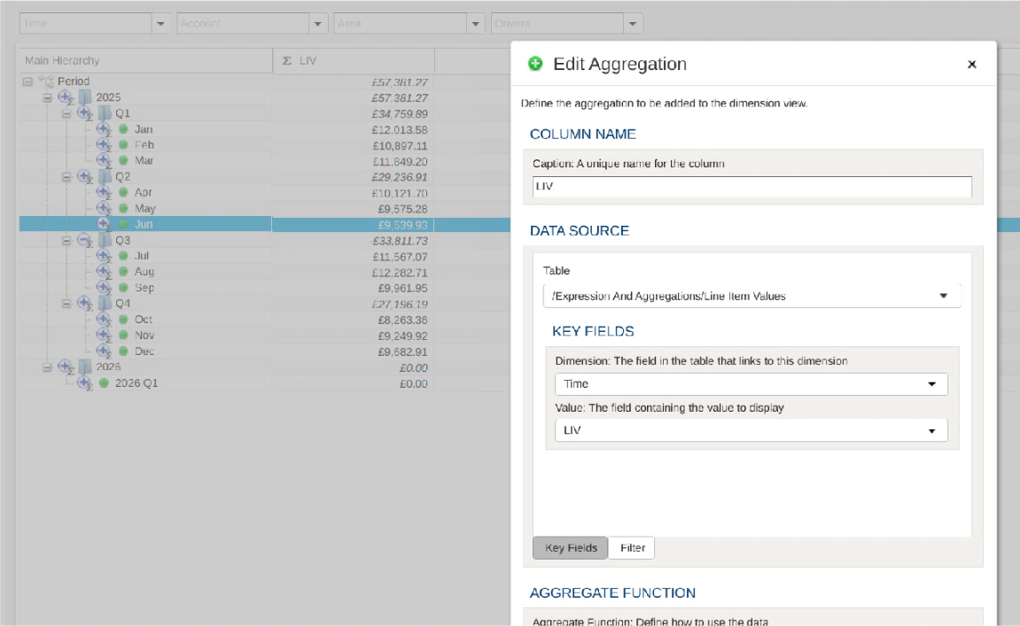
Aggregations can be filtered so that only items matching the filter are displayed. In the following image we have set up the aggregation to show values for a selected item in the ‘Account’ dimension.
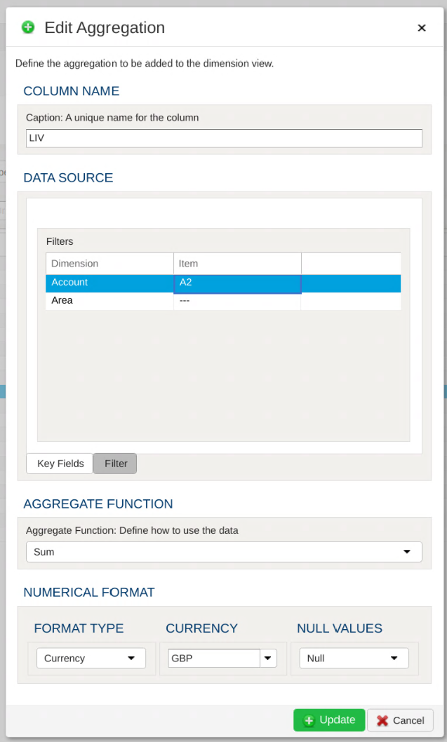
If these filters are left blank then the data can be filtered by using the dimension filter bar at the top of the screen, as can be seen in the following image:
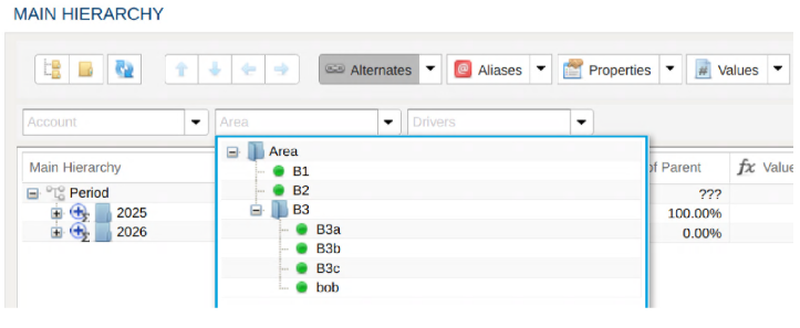
## Expressions
[Section titled “Expressions”](#expressions)
Using Expressions it is possible to display values which are calculated based on values from Aggregations displayed for the dimension. Expressions are built using mathematical formulae, which can contain many kinds of operators, and some special functions. see the [list of operators](https://mathjs.org/docs/expressions/syntax.html). The functions available are described below
## Functions
[Section titled “Functions”](#functions)
### Column(``)
[Section titled “Column(\)”](#columncolumn_name)
Fetch a value from a named column for the current row/node.
Below we see an example of an Expression being defined to display the result of multiplying the Line Item Value by 2.
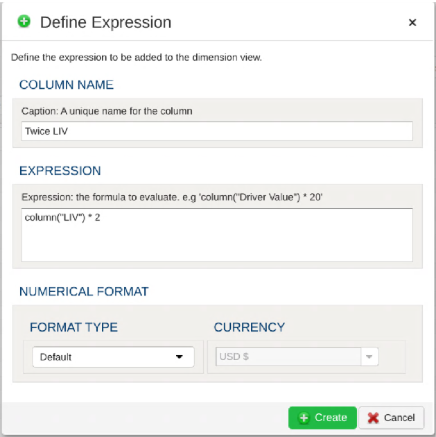
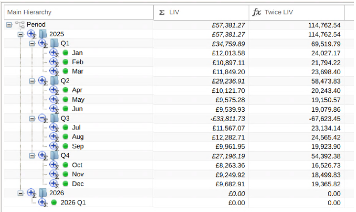
### Childcount()
[Section titled “Childcount()”](#childcount)
Returns the number of children for the current row/node. If the current row/node is a leaf item this will return 0.
In the following example this is being used to return the average value for the child nodes of a parent node.
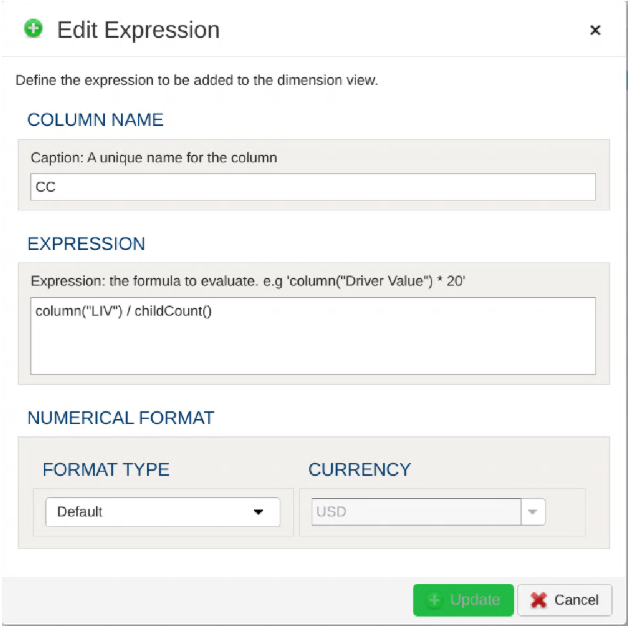
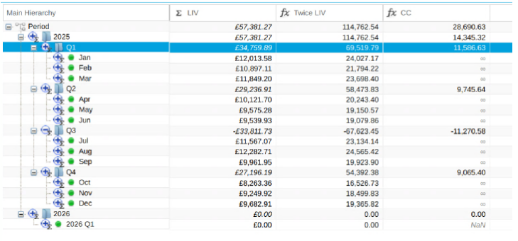
### Leafcount()
[Section titled “Leafcount()”](#leafcount)
Returns the number of leaf items found in the tree for the current row/node. If the current row/node is a leaf item this will return 1.
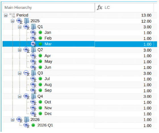
### Descendantcount()
[Section titled “Descendantcount()”](#descendantcount)
Returns the total number of items found in the tree for the current row/node. If the current row/node is a leaf item this will return 0.
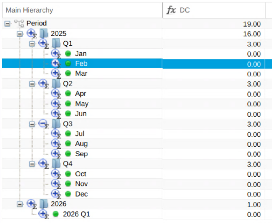
### Siblingcount()
[Section titled “Siblingcount()”](#siblingcount)
Returns the number of sibling items for the current row/node. The value returned includes the current node.
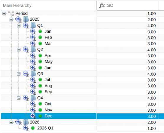
### Nodevalue(“``”,“``”)
[Section titled “Nodevalue(“\”,“\”)”](#nodevaluenode_namecolumn_name)
Returns the value from a named column for a named node. Here’s an example which is used to show the percentage of the “LIV” total for each row/node.

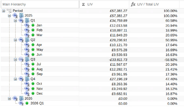
### Parentvalue(“\`”)
[Section titled “Columntextcompare(“\”)”](#columntextcomparecolumn_name-text)
Returns a numerical result representing if the text in a named column is greater than, less to, or equal to a provided value.
If the text from the column equals the provided text then this function returns 0.
If the text from the column is less than the provided text then this function returns -1.
If the text from the column is greater than the provided text then this function returns 0.
The following example compares the name of the Period to “Jun”
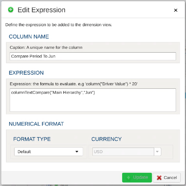
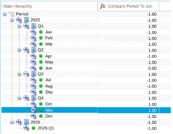
## Conditional Expressions
[Section titled “Conditional Expressions”](#conditional-expressions)
The examples shown above are fairly simplistic. By using conditionals within expressions it is possible to create more complex expressions. Within Expressions conditionals take the following form: `` ? `` : `` e.g ‘12 > 6 ? 1000: 0’
By combining expressions containing both conditionals and functions we can build more complex expressions, such as this example where 100,000 is added to a Line Item Value if the month is “Jun”
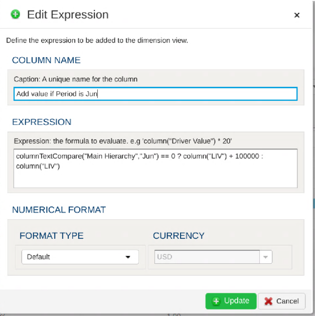
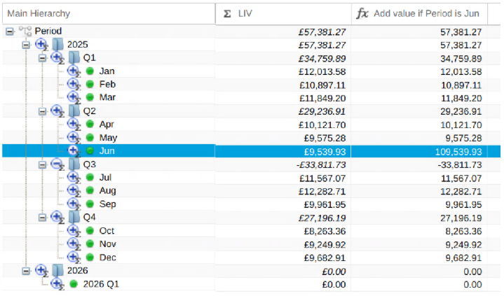
## Another Example: Simple Allocation
[Section titled “Another Example: Simple Allocation”](#another-example-simple-allocation)
This example shows the amount of a parent’s Line Item Value consumed by using the Resource Driver Value for a leaf node.
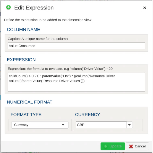
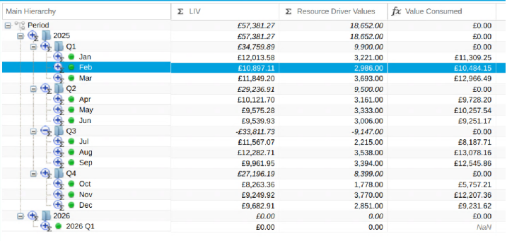
## Limitations:
[Section titled “Limitations:”](#limitations)
It is currently not possible to build Expressions which are based on values from other Expressions. Expressions can only be built using values from Aggregations.
# Getting Started with Dimensions
> Get started with PlaidCloud dimensions to organize hierarchical data with attributes, properties, and calculated values.
Dimensions are PlaidCloud’s hierarchies — the trees you use to organize cost centers, products, accounts, geography, time periods, or any other rolled-up structure. They’re the foundation that allocations, dashboards, and reports build on.
## When to Use a Dimension
[Section titled “When to Use a Dimension”](#when-to-use-a-dimension)
Reach for a dimension when you need to:
* Roll values up from leaves to parents (sum cost by department, then by region, then by company)
* Allocate from one set of rows to another based on a shared hierarchy (spread IT cost across business units)
* Slice a dashboard by a structure that’s deeper than a flat list (drill from continent → country → city)
* Apply the same grouping logic in multiple places — define the tree once, reference it everywhere
If your data is already flat and one-dimensional, you don’t need a dimension. A regular table is fine.
## How Dimensions Are Structured
[Section titled “How Dimensions Are Structured”](#how-dimensions-are-structured)
Every dimension has one **main hierarchy** — the canonical tree where every leaf is registered exactly once. On top of that, you can layer **alternate hierarchies** that re-roll-up the same leaves under different parents (e.g., the main tree groups cost centers by department, an alternate groups them by region).
Each node in the tree can carry properties, aliases, and values, so a hierarchy is more than just a tree of names — it’s a structure with metadata that allocations and reports can reference.
For the mechanics of creating, copying, sorting, and managing dimensions, see [Using Dimensions (Hierarchies)](/guides/dimensions/dimensions/).
## How Dimensions Get Loaded
[Section titled “How Dimensions Get Loaded”](#how-dimensions-get-loaded)
Dimensions are typically populated from a source table via a workflow:
* **Parent-Child format** — two columns (parent, child), one edge per row
* **Levels format** — one column per hierarchy level, one full path per row
See [Loading and unloading dimensions](/guides/dimensions/loading-unloading/) for the load process, and the [Dimension Load](/reference/workflow-steps/dimensions/dimension-load/) workflow step for the full set of options.
## What’s Next
[Section titled “What’s Next”](#whats-next)
* [Using Dimensions (Hierarchies)](/guides/dimensions/dimensions/) — full management reference
* [Function expressions](/guides/dimensions/function-expressions/) — calculated values inside a hierarchy
* [Loading and unloading](/guides/dimensions/loading-unloading/) — moving data in and out
* [Allocations](/guides/allocations/) — the main consumer of dimension structure
# Loading and Unloading Dimensions
> Load and unload dimension data in PlaidCloud including bulk imports, data refresh, and synchronization with external data sources.
Dimensions can be maintained from workflow operations by loading data. In addition, dimensional data can be flattened into tabular data and stored in tables. This is often useful for enriching reporting and analytics data.
## Loading Dimensions
[Section titled “Loading Dimensions”](#loading-dimensions)
Since dimensions represent hierarchical data structures, the load process must convey the relationships in the data. PlaidCloud supports two different data structures for loading dimensions:
* Parent-Child - The data is organized vertically with a *Parent* column and *Child* column defining each parent of a child throughout the structure
* Levels - The data is organized horizontally with each column representing a level in the hierarchy from left to right
In addition to structure, other dimension information can be included in the load process such as values, aliases, and properties.
See the Workflow Step for [Dimension Load](/reference/workflow-steps/dimensions/dimension-load) for more information.
## Unloading (exporting) Dimensions
[Section titled “Unloading (exporting) Dimensions”](#unloading-exporting-dimensions)
Exporting dimensions to tables supports two structural approaches:
* Parent-Child - The data is organized vertically with a *Parent* column and *Child* column defining each parent of a child throughout the structure
* Levels - The data is organized horizontally with each column representing a level in the hierarchy from left to right
Properties and values can also be included in the flattened tabular data.
See the Workflow Step for [Dimension Export](/reference/workflow-steps/dimensions/dimension-export) for more information.
# File Management
> Manage file storage accounts in PlaidCloud for importing and exporting data via CSV, Excel, Parquet, and other file formats.
PlaidCloud Documents — store, organize, search, and share files alongside your data and workflows. Documents can be sourced from any connected storage account and referenced in workflows.
# Account and Access Management
> Control access to PlaidCloud document accounts including permissions, backups, ownership settings, and start path configuration.
Control access to PlaidCloud document accounts — permissions, backups, ownership transfer, and start-path configuration so each account exposes only the relevant subtree of storage.
# Control Document Account Access
> Control who can access PlaidCloud document storage accounts by configuring permissions, roles, and access restrictions.
Four types of access restrictions are available for an account: Private, Workspace, Member Only, and Security Group. The type of restriction set for a user is editable at any time from the account form.
Note
None of the account access levels reveal the account credentials used to access the documents. Only account owners can view the credentials.
## Updating Account Access
[Section titled “Updating Account Access”](#updating-account-access)
1. Select `Document > Manage Accounts` within PlaidCloud
2. Enter the edit mode on the account you wish to change
3. Select the desired access level restriction located under `Security Model`
4. Select the Save button
Note
Depending on the selected Security Model, there will be different options for assigning which members or security groups are allowed access from the account list under Manage Accounts.
## Restriction Options
[Section titled “Restriction Options”](#restriction-options)
### All Workspace Members
[Section titled “All Workspace Members”](#all-workspace-members)
This access is the simplest since it provides access to all members of the workspace and does not require any additional assignment of members.
### Specific Members Only
[Section titled “Specific Members Only”](#specific-members-only)
This access setting requires assignment of each member to an account. This option is particularly useful when combined with the single sign-on option of assigning members based on a list of groups sent with the authentication. However, for workspaces with large numbers of members, this approach can often require more effort than desired, which is where security groups become useful. To choose specific members only:
1. Select the members icon from the Manage Accounts list
2. Drag the desired members from the `Unassigned Members` column on the left, to the `Assigned Members` column on the right
3. To remove members, do the opposite
4. Select the Save button
### Specific Security Groups Only
[Section titled “Specific Security Groups Only”](#specific-security-groups-only)
With this option, permission to access an account is granted to specific security groups rather than just individuals. With access restrictions relying on association with a security group or groups, the administration of accounts with much larger user counts becomes much simpler. To edit assigned groups:
1. Select the groups icon from the Manage Accounts list
2. Drag the desired groups from the `Unassigned Groups` column on the left, to the `Assigned Groups` column on the right
3. To remove groups, do the opposite
4. Select the Save button
### Remote Agents
[Section titled “Remote Agents”](#remote-agents)
PlaidLink agents will often use Document accounts to store files or move files among systems. To allow remote agents access to Document accounts, agents MUST have permission granted. This is a security feature to limit unwanted access to potentially sensitive information. To add agents:
1. Select the agent icon from the Manage Accounts list
2. Drag desired agents from the `Unassigned Agents` column on the left, to the `Assigned Agents` column on the right
3. To remove agents, do the opposite
4. Select the Save button
# Document Temporary Storage
> Manage temporary file storage in PlaidCloud document accounts for intermediate data processing and short-term file staging.
Temporary storage may sound counter-intuitive, but real-world use has shown it to be valuable. Typically, permanent storage is used to move large files between members or among other systems, and file cleanup in these storage locations often happens haphazardly, at best. This causes storage to fill with files that shouldn’t be there, eventually requiring manual cleanup.
Temporary storage is perfect for sharing or transferring these types of large files because the files are automatically deleted after 24 hours.
## To View Temporary Storage Options
[Section titled “To View Temporary Storage Options”](#to-view-temporary-storage-options)
1. Go To the `Document > Temp Share` in PlaidCloud
## Shared Temporary Storage
[Section titled “Shared Temporary Storage”](#shared-temporary-storage)
Shared temporary storage is viewable by all members of the workspace but is not viewable across workspaces. To access the shared temporary storage area, select the `Temp Share` menu and click `Workspace Temp Share` to display a table of files currently in the workspace’s Temp Share area.
### To Add New Files to a Shared Temporary Storage Location
[Section titled “To Add New Files to a Shared Temporary Storage Location”](#to-add-new-files-to-a-shared-temporary-storage-location)
1. Select the `Temp Share` menu along the top of the main Document page
2. Click `Workspace Temp Share`
3. Click `Browse` to browse locally stored items
4. Select the desired file and click `Open`
5. Click `Upload` to upload the file to the temporary storage location
### To Download Existing Files From Temporary Storage
[Section titled “To Download Existing Files From Temporary Storage”](#to-download-existing-files-from-temporary-storage)
1. Click on left-most icon, which represents the file type
### To Manually Delete a File
[Section titled “To Manually Delete a File”](#to-manually-delete-a-file)
1. Click the red delete icon to the left of the file name.
Additional details on file management can be found below under “File Explorer”.
## Personal Temporary Storage
[Section titled “Personal Temporary Storage”](#personal-temporary-storage)
Personal temporary storage is only viewable by the member to which the temp share belongs. This storage option is beneficial because it’s accessible across workspaces. This functionality makes it easy to move or use files across workspaces if the member is working in multiple workspaces simultaneously.
All members of the workspace can upload files to a members personal share as a dropbox.
### To Upload a File to Another Member’s Personal Share:
[Section titled “To Upload a File to Another Member’s Personal Share:”](#to-upload-a-file-to-another-members-personal-share)
1. Select the `Temp Share` menu along the top of the main Document page
2. Select `Drop File to Member Temp.` A list of members will be displayed.
3. Click the left-most icon associated with the member of your choosing
4. Click `Browse` to browse locally stored items
5. Select desired file and then click `Open`
6. Click `Upload` to upload the file to the member’s personal storage
Additional details on file uploading can be found below under “File Explorer”.
# Managing Document Account Backups
> Configure and manage backup settings for PlaidCloud document storage accounts to protect your files and ensure data recovery.
Document enables the backup of any account on a nightly basis. This feature permits backup across different cloud storage providers and on local systems. Essentially, any account is a valid target for the backup of another account.
Note
You cannot backup to the same account.
The backup process is not limited to a single backup destination. It is possible to have multiple redundant backup locations specified if this is a desired approach. For example, the backup of an internal server to another server may be one location with a second backup sent to Amazon S3 for off-site storage.
By using the prefix feature, it’s possible to have a single backup account contain the backups from multiple other accounts. Each account backup set begins its top level folder(s) with a different prefix, making it easy to distinguish the originating location and the restoration process. For example, if you have three different Document accounts but want to set their backup destination to the same location, using a prefix would allow all three accounts to properly backup without the fear of a name collision.
## Reviewing Current Backup Settings
[Section titled “Reviewing Current Backup Settings”](#reviewing-current-backup-settings)
1. Go to Document > Manage Accounts
2. Select the backup icon for the account you wish to review
## Creating a Backup Set
[Section titled “Creating a Backup Set”](#creating-a-backup-set)
1. Go to Document > Manage Accounts
2. Select the backup icon for the account for which to create a backup
3. Select the `New Backup Set` button
4. Complete the required fields
5. Select the `Create` button
The backup process is now scheduled to run nightly (US Time).
## Updating a Backup Set
[Section titled “Updating a Backup Set”](#updating-a-backup-set)
1. Go to Document > Manage Accounts
2. Select the backup icon for the account for which to edit a backup
3. Select the edit icon of the desired backup set
4. Adjust the desired information
5. Select the `Update` button
## Deleting a Backup Set
[Section titled “Deleting a Backup Set”](#deleting-a-backup-set)
1. Go to Document > Manage Accounts
2. Select the backup icon for the account for which to edit a backup
3. Select the delete icon of the desired backup set
4. Select the `Delete` button
Note
The backup sets already present will not be deleted but the backup process will no longer run. You can remove the existing backups using Document file and directory management processes.
# Managing Document Account Owners
> Assign and manage ownership of PlaidCloud document storage accounts to control administrative access and account settings.
The member who creates the account is assigned as the owner by default. However, Document accounts are designed to support multiple owners. This feature is helpful when a team is responsible for managing account access or when there is member turnover. Adding and removing owners is similar to adding and removing access permissions.
## Add or Remove Owners
[Section titled “Add or Remove Owners”](#add-or-remove-owners)
1. Go to `Document > Management Accounts` in PlaidCloud
2. Select the owners icon in the Manage Accounts list
3. Drag new owners from the `Unassigned Members` column on the left to the `Assigned Members` column on the right
4. To remove owners, do the opposite
5. Select the Save button
Because only owners have the ability to view and edit an account, account administration is set up with two levels:
* The member needs security access to view and manage accounts in general, and
* The member must be an owner of the account to view, manage, and change settings of accounts
Note
The list of accounts to manage will show a member only the accounts to which they are assigned as an account owner
# Using Start Paths in Document Accounts
> Configure start paths in PlaidCloud document accounts to control the default directory location when browsing file storage.
The account management form allows the configuration of the storage connection information and a start path. A start path allows those who use the account to begin browsing the directory structure further down the directory tree. This particular option is useful when you have multiple teams that need segregated file storage, but you only want one underlying storage service account.
The Start Path option in Document accounts is useful for the following reasons:
* When controlling access to sub-directories for specific teams and groups
* Granting access to only one bucket
For example, setting a start path of *teams/team\_1/* for the `Team 1` Document account *and teams/team\_2* for the `Team 2` Document account provides different start points on a shared account. When a member opens the Team 1 Document account they will begin file navigation inside *team/team\_1*. They will not be able to move up the tree and see anything above *teams/team\_1*.
Team 2 would have a similar restriction of not being able to navigate into Team 1’s area.
This provides the ability to restrict specific teams to lower levels of the tree while allowing other teams higher level access to the tree while not needing any additional cloud storage complexity like additional buckets or special permissions.
## Adding and Updating the Start Path
[Section titled “Adding and Updating the Start Path”](#adding-and-updating-the-start-path)
1. Go to Document > Manage Accounts
2. Select the account you wish to edit and enter the edit mode
3. Add a Start Path in the Start Path text field
4. Select the save button
## Start Path Format
[Section titled “Start Path Format”](#start-path-format)
The path always begins with the bucket name followed by the sub-directories.
```text
/folder1/folder2/
```
# Adding New Document Accounts
> Connect cloud and on-prem document storage to PlaidCloud — S3, GCS, Azure Blob, Google Drive, OneDrive, SFTP, WebDAV, and more.
Connect cloud and on-prem document storage to PlaidCloud — S3, Google Cloud Storage, Azure Blob, Google Drive, OneDrive, SFTP, WebDAV, and more. Each provider has its own credentials and connection flow.
# Add AWS S3 Account
> Add an AWS S3 storage account to PlaidCloud for importing and exporting data files using Amazon cloud object storage.
## AWS S3 Setup
[Section titled “AWS S3 Setup”](#aws-s3-setup)
These steps need to be completed within the AWS console.
1. Sign into or create an Amazon Web Services (AWS) account
2. Go to `All services > Storage > S3` in the console
3. Create a default or test bucket. Note the bucket name and region (e.g. `us-east-1`).
4. Go to `All Services > Security Identity & Compliance > IAM > Users` in the console
5. Select the `Create User` button
6. When prompted, enter a username and select `Access Key - Programmatic access` only. Select the `Next: Permissions` button.
7. Select the option box called `Attach existing policies directly`
8. In the filter search box type `s3`. When the list filters down to S3 related items select `AmazonS3FullAccess` by checking the box to the left. Select the `Next: Tags` button.
9. Skip this step by selecting the `Next: Review` button
10. Review the User settings and select `Create user`
11. Capture the keys generated for the user by downloading the CSV or copy/pasting the keys somewhere for use later. You will not be able to retrieve this key again so keep track of it. If you need to regenerate a key simply go back to step 5 above.
You should now have everything you need to add your S3 account to PlaidCloud Document.
## PlaidCloud Document Setup
[Section titled “PlaidCloud Document Setup”](#plaidcloud-document-setup)
1. Sign into PlaidCloud
2. Select the workspace that the new Document account will reside
3. Go to `Document > Manage Accounts`
4. Select the `+ New Account` button
5. Select `Amazon S3` as the Service Type
6. Fill in a name and description
7. Enter the bucket name and optional path prefix into the **Start Path** field (e.g. `my-bucket` or `my-bucket/data`). The first path segment is the bucket name.
8. Select an appropriate **Security Model** for your use case. Leave it `Private` if unsure.
9. Paste the **Access Key** created in step 11 above into the Access Key ID field under Auth Credentials
10. Paste the **Secret Key** created in step 11 above into the Secret Access Key field under Auth Credentials
11. Enter the **Region** for your bucket (e.g. `us-east-1`, `eu-west-1`). If left blank, defaults to `us-east-2`.
12. Select the Save button and your new Document account is live
# Add Azure Blob Storage Account
> Add an Azure Blob Storage account to PlaidCloud for importing and exporting data files using Microsoft Azure cloud object storage.
## Azure Blob Storage Setup
[Section titled “Azure Blob Storage Setup”](#azure-blob-storage-setup)
These steps need to be completed within the Azure portal.
1. Sign in to the [Azure portal](https://portal.azure.com)
2. Navigate to **Storage accounts** and select or create a storage account
3. In the left sidebar under **Security + networking**, select **Access keys**
4. Copy the **Storage account name** and one of the **Key** values. Save both for the PlaidCloud Document setup below.
5. Navigate to **Containers** under **Data storage** and create a container if one does not already exist. Note the container name.
You should now have everything you need to add your Azure Blob Storage account to PlaidCloud Document.
## PlaidCloud Document Setup
[Section titled “PlaidCloud Document Setup”](#plaidcloud-document-setup)
1. Sign into PlaidCloud
2. Select the workspace that the new Document account will reside
3. Go to `Document > Manage Accounts`
4. Select the `+ New Account` button
5. Select `Azure Blob Storage` as the Service Type
6. Fill in a name and description
7. Enter the container name and optional path prefix into the **Start Path** field (e.g. `my-container/data`). The first path segment is the container name.
8. Select an appropriate **Security Model** for your use case. Leave it `Private` if unsure.
9. Paste the **Storage account name** into the Account Name field under Auth Credentials
10. Paste the **Key** into the Account Key field under Auth Credentials
11. Select the Save button and your new Document account is live
# Add Azure Data Lake Gen2 Account
> Add an Azure Data Lake Storage Gen2 account to PlaidCloud for importing and exporting data files using hierarchical namespace storage on Azure.
## Azure Data Lake Gen2 Setup
[Section titled “Azure Data Lake Gen2 Setup”](#azure-data-lake-gen2-setup)
Azure Data Lake Storage Gen2 is built on top of Azure Blob Storage with a hierarchical namespace enabled. These steps need to be completed within the Azure portal.
1. Sign in to the [Azure portal](https://portal.azure.com)
2. Navigate to **Storage accounts** and select or create a storage account that has **Hierarchical namespace** enabled
3. In the left sidebar under **Security + networking**, select **Access keys**
4. Copy the **Storage account name** and one of the **Key** values. Save both for the PlaidCloud Document setup below.
5. Navigate to **Containers** under **Data storage** and create a filesystem (container) if one does not already exist. Note the filesystem name.
You should now have everything you need to add your Azure Data Lake Gen2 account to PlaidCloud Document.
## PlaidCloud Document Setup
[Section titled “PlaidCloud Document Setup”](#plaidcloud-document-setup)
1. Sign into PlaidCloud
2. Select the workspace that the new Document account will reside
3. Go to `Document > Manage Accounts`
4. Select the `+ New Account` button
5. Select `Azure Data Lake Gen2` as the Service Type
6. Fill in a name and description
7. Enter the filesystem name and optional path prefix into the **Start Path** field (e.g. `my-filesystem/data`). The first path segment is the filesystem name.
8. Select an appropriate **Security Model** for your use case. Leave it `Private` if unsure.
9. Paste the **Storage account name** into the Account Name field under Auth Credentials
10. Paste the **Key** into the Account Key field under Auth Credentials
11. Select the Save button and your new Document account is live
# Add Backblaze B2 Account
> Add a Backblaze B2 storage account to PlaidCloud for importing and exporting data files using affordable cloud object storage.
## Backblaze B2 Setup
[Section titled “Backblaze B2 Setup”](#backblaze-b2-setup)
These steps need to be completed within the Backblaze B2 console.
1. Sign in to the [Backblaze B2 console](https://secure.backblaze.com/b2_buckets.htm)
2. Navigate to **Buckets** and create a bucket if one does not already exist. Note the bucket name.
3. Navigate to **App Keys**
4. Select **Add a New Application Key**
5. Give the key a name, select the bucket it should have access to, and choose the appropriate permissions (read and write)
6. Select **Create New Key**
7. Copy the **keyID** (this is your Access Key) and **applicationKey** (this is your Secret Key). Save both for the PlaidCloud Document setup below. The application key is only shown once.
8. Note the **S3 Endpoint** for your bucket’s region. It follows the pattern `https://s3.{region}.backblazeb2.com` (e.g. `https://s3.us-west-004.backblazeb2.com`). This can be found on the bucket details page.
You should now have everything you need to add your Backblaze B2 account to PlaidCloud Document.
## PlaidCloud Document Setup
[Section titled “PlaidCloud Document Setup”](#plaidcloud-document-setup)
1. Sign into PlaidCloud
2. Select the workspace that the new Document account will reside
3. Go to `Document > Manage Accounts`
4. Select the `+ New Account` button
5. Select `Backblaze B2` as the Service Type
6. Fill in a name and description
7. Enter the **Start Path** as your S3-compatible endpoint followed by the bucket name: `https://s3.us-west-004.backblazeb2.com/my-bucket`
8. Enter the **Region** for your bucket (e.g. `us-west-004`)
9. Select an appropriate **Security Model** for your use case. Leave it `Private` if unsure.
10. Paste the **keyID** into the Access Key ID field under Auth Credentials
11. Paste the **applicationKey** into the Secret Access Key field under Auth Credentials
12. Select the Save button and your new Document account is live
# Add Cloudflare R2 Account
> Add a Cloudflare R2 storage account to PlaidCloud for importing and exporting data files using Cloudflare's zero-egress-fee object storage.
## Cloudflare R2 Setup
[Section titled “Cloudflare R2 Setup”](#cloudflare-r2-setup)
These steps need to be completed within the Cloudflare dashboard.
1. Sign in to the [Cloudflare dashboard](https://dash.cloudflare.com)
2. Select your account, then navigate to **R2 Object Storage** in the left sidebar
3. Create a bucket if one does not already exist. Note the bucket name.
4. Navigate to **R2 Object Storage > Manage R2 API Tokens**
5. Select **Create API Token**
6. Give the token a name, select the bucket(s) it should have access to, and choose **Object Read & Write** permissions
7. Select **Create API Token**
8. Copy the **Access Key ID** and **Secret Access Key**. Save both for the PlaidCloud Document setup below. The secret is only shown once.
9. Note the **S3 API endpoint** for your account. It follows the pattern `https://{account_id}.r2.cloudflarestorage.com` and is shown on the R2 overview page.
You should now have everything you need to add your Cloudflare R2 account to PlaidCloud Document.
## PlaidCloud Document Setup
[Section titled “PlaidCloud Document Setup”](#plaidcloud-document-setup)
1. Sign into PlaidCloud
2. Select the workspace that the new Document account will reside
3. Go to `Document > Manage Accounts`
4. Select the `+ New Account` button
5. Select `Cloudflare R2` as the Service Type
6. Fill in a name and description
7. Enter the **Start Path** as your R2 endpoint followed by the bucket name: `https://{account_id}.r2.cloudflarestorage.com/my-bucket`
8. The **Region** field can be set to `auto` or left blank — R2 automatically selects the closest region
9. Select an appropriate **Security Model** for your use case. Leave it `Private` if unsure.
10. Paste the **Access Key ID** into the Access Key ID field under Auth Credentials
11. Paste the **Secret Access Key** into the Secret Access Key field under Auth Credentials
12. Select the Save button and your new Document account is live
# Add DigitalOcean Spaces Account
> Add a DigitalOcean Spaces storage account to PlaidCloud for importing and exporting data files using DigitalOcean's S3-compatible object storage.
## Digitalocean Spaces Setup
[Section titled “Digitalocean Spaces Setup”](#digitalocean-spaces-setup)
These steps need to be completed within the DigitalOcean control panel.
1. Sign in to the [DigitalOcean Control Panel](https://cloud.digitalocean.com)
2. Navigate to **Spaces Object Storage** in the left sidebar
3. Create a Space if one does not already exist. Note the Space name and region (e.g. `nyc3`).
4. Navigate to **API > Spaces Keys** (under the Tokens section)
5. Select **Generate New Key**
6. Give the key a name
7. Copy the **Key** (Access Key) and **Secret**. Save both for the PlaidCloud Document setup below. The secret is only shown once.
8. Note the endpoint URL for your Space’s region. It follows the pattern `https://{region}.digitaloceanspaces.com` (e.g. `https://nyc3.digitaloceanspaces.com`)
You should now have everything you need to add your DigitalOcean Spaces account to PlaidCloud Document.
## PlaidCloud Document Setup
[Section titled “PlaidCloud Document Setup”](#plaidcloud-document-setup)
1. Sign into PlaidCloud
2. Select the workspace that the new Document account will reside
3. Go to `Document > Manage Accounts`
4. Select the `+ New Account` button
5. Select `DigitalOcean Spaces` as the Service Type
6. Fill in a name and description
7. Enter the **Start Path** as the endpoint URL followed by the Space name: `https://nyc3.digitaloceanspaces.com/my-space`
8. Enter the **Region** (e.g. `nyc3`, `sfo3`, `ams3`)
9. Select an appropriate **Security Model** for your use case. Leave it `Private` if unsure.
10. Paste the **Key** into the Access Key ID field under Auth Credentials
11. Paste the **Secret** into the Secret Access Key field under Auth Credentials
12. Select the Save button and your new Document account is live
# Add FTP Account
> Add an FTP (File Transfer Protocol) account to PlaidCloud for importing and exporting data files using traditional FTP servers.
## FTP Server Setup
[Section titled “FTP Server Setup”](#ftp-server-setup)
Ensure the following are available from your FTP server administrator:
1. The **FTP server URL** (e.g. `ftp://ftp.yourcompany.com` or `ftp://192.168.1.100`)
2. A **username** with access to the target directory
3. A **password** for authentication
Note
FTP transmits credentials and data in plain text. For production use, consider SFTP instead which encrypts all traffic over SSH. Use FTP only when connecting to legacy systems that do not support SFTP.
You should now have everything you need to add your FTP account to PlaidCloud Document.
## PlaidCloud Document Setup
[Section titled “PlaidCloud Document Setup”](#plaidcloud-document-setup)
1. Sign into PlaidCloud
2. Select the workspace that the new Document account will reside
3. Go to `Document > Manage Accounts`
4. Select the `+ New Account` button
5. Select `FTP` as the Service Type
6. Fill in a name and description
7. Enter the **FTP server URL** into the **Start Path** field (e.g. `ftp://ftp.yourcompany.com`)
8. Select an appropriate **Security Model** for your use case. Leave it `Private` if unsure.
9. Enter the **username** into the Username field under Auth Credentials
10. Enter the **password** into the Password field under Auth Credentials
11. Select the Save button and your new Document account is live
# Add Google Cloud Storage Account
> Add a Google Cloud Storage account to PlaidCloud for importing and exporting data files using Google cloud object storage.
## Google Cloud Setup
[Section titled “Google Cloud Setup”](#google-cloud-setup)
These steps need to be completed within Google Cloud Platform
1. Sign into or create a Google Cloud Platform account
2. Select or create a project where the Google Cloud Storage account will reside
3. Go to `Cloud Storage > Browser` in the Google Cloud Platform console
4. Create a default or test bucket
5. Go To `IAM & Admin > Service Accounts` in the Google Cloud Platform console
6. Select the `+ Create Service Account` button
7. Complete the service account information and create the account
8. Find the service account just created in the list of service accounts and select `Manage Keys` from the context menu on the right
9. Under the `Add Key` menu, select `Create a Key`
10. When prompted, select JSON format for the key. This will generate the key and automatically download it to your desktop. You will not be able to retrieve this key again so keep track of it. If you need to regenerate a key simply go back to step 8 above.
11. Go to `IAM & Admin > IAM` in the Google Cloud Platform console
12. Find the service account you just created and click on the edit permissions icon
13. Add `Storage Admin` and `Storage Transfer Admin` rights for the service account and save. Note less permissive rights can be assigned but this will impact the functionality available through Document.
You should now have everything you need to add your GCS account to PlaidCloud Document.
## PlaidCloud Document Setup
[Section titled “PlaidCloud Document Setup”](#plaidcloud-document-setup)
1. Sign into PlaidCloud
2. Select the workspace that the new Document account will reside
3. Go to `Document > Manage Accounts`
4. Select the `+ New Account` button
5. Select `Google Cloud Storage` as the Service Type
6. Fill in a name and description
7. Enter the bucket name and optional path prefix into the **Start Path** field (e.g. `my-bucket` or `my-bucket/data`). The first path segment is the bucket name.
8. Select an appropriate **Security Model** for your use case. Leave it `Private` if unsure.
9. Open the Service Account JSON key file you downloaded in step 10 above and copy the entire contents
10. Paste the contents into the **System User JSON Key** field under Auth Credentials
11. Select the Save button and your new Document account is live
# Add Google Drive Account
> Add a Google Drive storage account to PlaidCloud for importing and exporting data files using Google Drive cloud storage.
## Google Drive Setup
[Section titled “Google Drive Setup”](#google-drive-setup)
These steps need to be completed within the Google Cloud Console to create a service account that PlaidCloud can use to access Google Drive.
### Create a Google Cloud Project
[Section titled “Create a Google Cloud Project”](#create-a-google-cloud-project)
1. Sign in to the [Google Cloud Console](https://console.cloud.google.com)
2. Create a new project or select an existing one
### Enable the Google Drive API
[Section titled “Enable the Google Drive API”](#enable-the-google-drive-api)
1. Navigate to **APIs & Services > Library**
2. Search for **Google Drive API**
3. Select it and click **Enable**
### Create a Service Account
[Section titled “Create a Service Account”](#create-a-service-account)
1. Navigate to **APIs & Services > Credentials**
2. Select **+ Create Credentials > Service account**
3. Enter a name for the service account (e.g. `plaidcloud-drive`)
4. Select **Create and Continue**
5. Optionally grant roles (e.g. **Viewer** for read-only, or **Editor** for read/write). Select **Continue**.
6. Select **Done**
### Generate a Service Account Key
[Section titled “Generate a Service Account Key”](#generate-a-service-account-key)
1. In the **Service Accounts** list, select the service account you just created
2. Navigate to the **Keys** tab
3. Select **Add Key > Create new key**
4. Choose **JSON** format and select **Create**
5. A JSON key file will download. Save this file securely — it contains the credentials PlaidCloud will use.
### Share Drive Content With the Service Account
[Section titled “Share Drive Content With the Service Account”](#share-drive-content-with-the-service-account)
1. Copy the service account’s email address (e.g. `plaidcloud-drive@your-project.iam.gserviceaccount.com`)
2. In Google Drive, share the folder(s) you want PlaidCloud to access with this email address, granting **Editor** access
You should now have everything you need to add your Google Drive account to PlaidCloud Document.
## PlaidCloud Document Setup
[Section titled “PlaidCloud Document Setup”](#plaidcloud-document-setup)
1. Sign into PlaidCloud
2. Select the workspace that the new Document account will reside
3. Go to `Document > Manage Accounts`
4. Select the `+ New Account` button
5. Select `Google Drive` as the Service Type
6. Fill in a name and description
7. Enter the shared folder path into the **Start Path** field, or leave it blank to access all shared content
8. Select an appropriate **Security Model** for your use case. Leave it `Private` if unsure.
9. Paste the entire contents of the JSON key file into the OAuth2 Credentials JSON field under Auth Credentials
10. Select the Save button and your new Document account is live
# Add Linode Object Storage Account
> Add a Linode (Akamai) Object Storage account to PlaidCloud for importing and exporting data files using Linode's S3-compatible cloud storage.
## Linode Object Storage Setup
[Section titled “Linode Object Storage Setup”](#linode-object-storage-setup)
These steps need to be completed within the Linode Cloud Manager.
1. Sign in to the [Linode Cloud Manager](https://cloud.linode.com)
2. Navigate to **Object Storage** in the left sidebar
3. Create a bucket if one does not already exist. Note the bucket name (called **label**) and region (e.g. `us-east-1`).
4. Navigate to **Object Storage > Access Keys**
5. Select **Create Access Key**
6. Give the key a label and select the bucket(s) it should have access to with read/write permissions
7. Select **Create Access Key**
8. Copy the **Access Key** and **Secret Key**. Save both for the PlaidCloud Document setup below. The secret is only shown once.
9. Note the endpoint URL for your bucket’s region. It follows the pattern `https://{region}.linodeobjects.com` (e.g. `https://us-east-1.linodeobjects.com`)
You should now have everything you need to add your Linode Object Storage account to PlaidCloud Document.
## PlaidCloud Document Setup
[Section titled “PlaidCloud Document Setup”](#plaidcloud-document-setup)
1. Sign into PlaidCloud
2. Select the workspace that the new Document account will reside
3. Go to `Document > Manage Accounts`
4. Select the `+ New Account` button
5. Select `Linode Object Storage` as the Service Type
6. Fill in a name and description
7. Enter the **Start Path** as the endpoint URL followed by the bucket name: `https://us-east-1.linodeobjects.com/my-bucket`
8. Enter the **Region** (e.g. `us-east-1`)
9. Select an appropriate **Security Model** for your use case. Leave it `Private` if unsure.
10. Paste the **Access Key** into the Access Key ID field under Auth Credentials
11. Paste the **Secret Key** into the Secret Access Key field under Auth Credentials
12. Select the Save button and your new Document account is live
# Add MinIO Account
> Add a MinIO storage account to PlaidCloud for importing and exporting data files using self-hosted S3-compatible object storage.
## Minio Setup
[Section titled “Minio Setup”](#minio-setup)
These steps need to be completed within the MinIO Console or via the `mc` CLI.
1. Sign in to the MinIO Console (e.g. `https://your-minio-host:9001`)
2. Navigate to **Buckets** and create a bucket if one does not already exist. Note the bucket name.
3. Navigate to **Identity > Users** (or **Access Keys**)
4. Create a new user or service account with read/write access to the target bucket
5. Copy the **Access Key** and **Secret Key** generated for the user. Save both for the PlaidCloud Document setup below.
6. Note the MinIO endpoint URL (e.g. `https://play.min.io` or `https://minio.yourcompany.com`)
You should now have everything you need to add your MinIO account to PlaidCloud Document.
## PlaidCloud Document Setup
[Section titled “PlaidCloud Document Setup”](#plaidcloud-document-setup)
1. Sign into PlaidCloud
2. Select the workspace that the new Document account will reside
3. Go to `Document > Manage Accounts`
4. Select the `+ New Account` button
5. Select `MinIO` as the Service Type
6. Fill in a name and description
7. Enter the **Start Path** as your MinIO endpoint URL followed by the bucket name and optional prefix: `https://minio.yourcompany.com/my-bucket/optional/prefix`
8. Enter the **Region** if your MinIO deployment uses regions; otherwise leave blank
9. Select an appropriate **Security Model** for your use case. Leave it `Private` if unsure.
10. Paste the **Access Key** into the Access Key ID field under Auth Credentials
11. Paste the **Secret Key** into the Secret Access Key field under Auth Credentials
12. Select the Save button and your new Document account is live
# Add OneDrive Account
> Add a Microsoft OneDrive storage account to PlaidCloud for importing and exporting data files using OneDrive cloud storage.
## Onedrive Setup
[Section titled “Onedrive Setup”](#onedrive-setup)
These steps need to be completed within the Azure portal to register an application and obtain the credentials PlaidCloud needs to access OneDrive.
### Register an Application in Azure
[Section titled “Register an Application in Azure”](#register-an-application-in-azure)
1. Sign in to the [Azure portal](https://portal.azure.com) and navigate to **Microsoft Entra ID**.
2. In the left sidebar, select **App registrations**.
3. Click **+ New registration**.
4. Enter a name for the application (e.g., `PlaidCloud`).
5. Under **Supported account types**, select the option that matches your organization:
* **Accounts in this organizational directory only** — for a single-tenant setup (most common)
* **Accounts in any organizational directory** — for multi-tenant access
6. Leave the **Redirect URI** blank.
7. Click **Register**.
### Copy the Client ID and Tenant ID
[Section titled “Copy the Client ID and Tenant ID”](#copy-the-client-id-and-tenant-id)
After registration, you will land on the application overview page.
1. Copy the **Application (client) ID** — this is your **Client ID**. Save it for the PlaidCloud Document setup below.
2. Copy the **Directory (tenant) ID** — this is your **Tenant ID**. Save it as well.
Both values are displayed on the application overview page immediately after registration.
### Create a Client Secret
[Section titled “Create a Client Secret”](#create-a-client-secret)
1. In the left sidebar, select **Certificates & secrets** under **Manage**.
2. Click **+ New client secret**.
3. Enter a description (e.g., `PlaidCloud`) and choose an expiration period.
4. Click **Add**.
5. Copy the **Value** of the newly created secret immediately — this is your **Client Secret**. It will not be shown again after you leave this page.
### Grant API Permissions
[Section titled “Grant API Permissions”](#grant-api-permissions)
1. In the left sidebar, select **API permissions** under **Manage**.
2. Click **+ Add a permission**.
3. Select **Microsoft Graph**.
4. Add the following permissions, selecting the type indicated for each:
* `Directory.ReadWrite.All` (Application) — Read and write directory data
* `Files.Read.All` (Application) — Read files in all site collections
* `Files.ReadWrite.All` (Application) — Read and write files in all site collections
* `Sites.ReadWrite.All` (Application) — Read and write items in all site collections
* `User.Read` (Delegated) — Sign in and read user profile
* `User.Read.All` (Application) — Read all users’ full profiles
5. Click **Add permissions**.
6. Click **Grant admin consent for \[your organization]** and confirm.
***
### Find the Onedrive Drive Path (start Path)
[Section titled “Find the Onedrive Drive Path (start Path)”](#find-the-onedrive-drive-path-start-path)
The **Start Path** in PlaidCloud Document controls which drive or folder in OneDrive is used as the root for the account.
In the most common scenario, the registered application has access to multiple drives or SharePoint sites. In this case the Start Path must begin with the name of the drive or site. For most OneDrive for Business accounts this is simply:
```text
Documents
```
To target a specific subfolder within that drive, append the folder path:
```text
Documents/Finance
Documents/Shared/Data
```
Note
If the application only has access to a single drive, the Start Path can be left blank to use the root of that drive. When in doubt, start with `Documents` as the drive name.
***
You should now have everything you need to add your OneDrive account to PlaidCloud Document.
## PlaidCloud Document Setup
[Section titled “PlaidCloud Document Setup”](#plaidcloud-document-setup)
1. Sign into PlaidCloud
2. Select the workspace that the new Document account will reside
3. Go to `Document > Manage Accounts`
4. Select the `+ New Account` button
5. Select `OneDrive` as the Service Type
6. Fill in a name and description
7. Enter the folder path identified above into the **Start Path** field, or leave it blank to use the root of the drive
8. Select an appropriate **Security Model** for your use case. Leave it `Private` if unsure.
9. Paste the **Client ID** copied from the Azure app registration into the Public Key/User text field under Auth Credentials
10. Paste the **Client Secret** copied from the Azure app registration into the Private Key/Password text field under Auth Credentials
11. Paste the **Tenant ID** copied from the Azure app registration into the Tenant ID field under Auth Credentials
12. Select the Save button and your new Document account is live
# Add SFTP Account
> Add an SFTP (Secure File Transfer Protocol) account to PlaidCloud for importing and exporting data files using SSH-based file transfer.
## SFTP Server Setup
[Section titled “SFTP Server Setup”](#sftp-server-setup)
Ensure the following are available from your SFTP server administrator:
1. The **hostname or IP address** of the SFTP server
2. The **SSH port** (default is `22`)
3. A **username** with access to the target directory
4. Either a **password** or an **SSH private key** for authentication
5. Optionally, the **server’s SSH host key fingerprint** for strict host verification
You should now have everything you need to add your SFTP account to PlaidCloud Document.
## PlaidCloud Document Setup
[Section titled “PlaidCloud Document Setup”](#plaidcloud-document-setup)
1. Sign into PlaidCloud
2. Select the workspace that the new Document account will reside
3. Go to `Document > Manage Accounts`
4. Select the `+ New Account` button
5. Select `Secure File Transfer (SFTP)` as the Service Type
6. Fill in a name and description
7. Enter the remote directory path into the **Start Path** field (e.g. `/data/uploads`)
8. Select an appropriate **Security Model** for your use case. Leave it `Private` if unsure.
9. Enter the **username** into the Public Key/User field under Auth Credentials
10. Enter the **password** into the Private Key/Password field under Auth Credentials
11. Navigate to the **SSH Config** tab
12. Enter the **Host or IP Address** of the SFTP server
13. Enter the **SSH Connection Port** (default `22`)
14. If using key-based authentication instead of a password, paste the **RSA Private Key** into the RSA Private Key field. When a private key is provided, it takes precedence over the password.
15. Optionally paste the **Remote Server RSA Fingerprint** for strict host key verification. Leave blank to auto-fill on first connection.
16. Select the Save button and your new Document account is live
Note
You can test the SSH connection using the **Test SSH Connection** button on the SSH Config tab before saving.
# Add Wasabi Hot Storage Account
> Add a Wasabi Hot Storage account to PlaidCloud for importing and exporting data files using cost-effective cloud storage.
## Wasabi Hot Storage Setup
[Section titled “Wasabi Hot Storage Setup”](#wasabi-hot-storage-setup)
These steps need to be completed within the Wasabi Hot Storage console
1. Sign into or create a Wasabi Hot Storage account
2. Go to `Buckets` in the console
3. Create a default or test bucket
4. Go to Users in the console
5. Select the `Create User` button
6. When prompted, enter a username and select `Programmatic (create API key)` user
7. Skip the group assignment. Select the `Next` button
8. Select the plus icon next to the `WasabiFullAccess` policy to attach the policy to the user. Select the `Next` button.
9. Review the User settings and select `Create User`
10. Capture the keys generated for the user by downloading the CSV or copy/pasting the keys somewhere for use later. You will not be able to retrieve this key again so keep track of it. If you need to regenerate a key simply go back to step 5 above.
You should now have everything you need to add your Wasabi account to PlaidCloud Document.
## PlaidCloud Document Setup
[Section titled “PlaidCloud Document Setup”](#plaidcloud-document-setup)
1. Sign into PlaidCloud
2. Select the workspace that the new Document account will reside
3. Go to `Document > Manage Accounts`
4. Select the `+ New Account` button
5. Select `Wasabi Hot Storage` as the Service Type
6. Fill in a name and description
7. Enter the bucket name and optional path prefix into the **Start Path** field (e.g. `my-bucket` or `my-bucket/data`). The first path segment is the bucket name.
8. Select an appropriate **Security Model** for your use case. Leave it `Private` if unsure.
9. Paste the **Access Key** created in step 10 above into the Access Key ID field under Auth Credentials
10. Paste the **Secret Key** created in step 10 above into the Secret Access Key field under Auth Credentials
11. Enter the **Region** if your Wasabi account uses a specific region; otherwise leave blank
12. Select the Save button and your new Document account is live
# Add WebDAV Account
> Add a WebDAV storage account to PlaidCloud for importing and exporting data files using WebDAV-compatible servers such as Nextcloud, ownCloud, or Apache.
## Webdav Server Setup
[Section titled “Webdav Server Setup”](#webdav-server-setup)
Ensure the following are available from your WebDAV server administrator:
1. The **WebDAV endpoint URL** (e.g. `https://nextcloud.yourcompany.com/remote.php/dav/files/username/`)
2. A **username** with access to the target directory
3. A **password** or app-specific password for authentication
Note
Many cloud services expose a WebDAV interface. For example, Nextcloud uses `https://your-server/remote.php/dav/files/{username}/` and ownCloud uses `https://your-server/remote.php/webdav/`. Check your provider’s documentation for the correct URL.
You should now have everything you need to add your WebDAV account to PlaidCloud Document.
## PlaidCloud Document Setup
[Section titled “PlaidCloud Document Setup”](#plaidcloud-document-setup)
1. Sign into PlaidCloud
2. Select the workspace that the new Document account will reside
3. Go to `Document > Manage Accounts`
4. Select the `+ New Account` button
5. Select `WebDAV` as the Service Type
6. Fill in a name and description
7. Enter the full **WebDAV endpoint URL** into the **Start Path** field (e.g. `https://nextcloud.yourcompany.com/remote.php/dav/files/username/`)
8. Select an appropriate **Security Model** for your use case. Leave it `Private` if unsure.
9. Enter the **username** into the Username field under Auth Credentials
10. Enter the **password** into the Password field under Auth Credentials
11. Select the Save button and your new Document account is live
# Searching Documents
> Find files in a PlaidCloud Document account using inline search with live progress, advanced filters, and reveal-in-folder.
## Description
[Section titled “Description”](#description)
The Document browser includes a search bar at the top of the file list. Searches run live against the connected backend (S3, Azure Blob, Google Drive, OneDrive, etc.) so results reflect the current state of the account, not a stale index.
## Run a Search
[Section titled “Run a Search”](#run-a-search)
1. Open a Document account
2. Click in the **Search files…** field at the top of the file list
3. Type a name pattern
4. Watch results stream into the file list
Press `Esc` or click the clear icon at the end of the field to exit search mode and return to the regular file list. The status line below the field shows how many folders have been scanned and how many matches have been found.
## Advanced Filters
[Section titled “Advanced Filters”](#advanced-filters)
Click `Advanced` next to the search field to show the filter row. Combine any of these filters with the name pattern:
* **Ext:** — comma-separated extensions, e.g. `pdf,xlsx`. No spaces.
* **Kind:** — `Files & folders` (default), `Files only`, or `Folders only`.
* **Size (bytes):** — minimum and/or maximum size.
* **Modified:** — on/after date and on/before date, both as `YYYY-MM-DD`.
Filters apply on top of the name pattern. Click `Clear` to wipe the query and all filters.
## Highlighting and Reveal
[Section titled “Highlighting and Reveal”](#highlighting-and-reveal)
* While the search is running, results stream in arrival order so you can act on early matches without waiting.
* Once the stream completes, the file list re-sorts by name and the matched substring is highlighted in each row.
* Right-click any result and select `Reveal in folder` to jump to the file in its containing directory and exit search mode.
## Searching Across Backends
[Section titled “Searching Across Backends”](#searching-across-backends)
Search uses the storage backend’s own search API where one is available, so results match what you’d see in the backend’s native UI:
* **Google Drive** — uses the Drive API.
* **OneDrive / SharePoint** — uses Microsoft Graph.
For object stores (S3 and S3-compatible, Azure Blob, GCS, etc.) PlaidCloud crawls the configured paths in parallel.
Note
Each user is rate-limited to a small number of concurrent searches per account so a heavy search won’t starve other users. If you hit the limit the search bar reports an error — wait for one of your other searches to finish and try again.
# Using Document Accounts
> Browse, upload, search, and manage files in PlaidCloud Document storage using the two-pane file explorer.
The Document browser is a two-pane split view: the folder tree on the left, the file list on the right. Most operations are available from a right-click menu in either pane. The right-click menu shows different options depending on whether a folder, a file, or empty space is selected.
The root of an account is itself a viewable, droppable folder — clicking it shows everything at the top level and accepts dropped uploads.
**To open the file explorer:**
1. Go to **Document > Shared Accounts** (or **Private Accounts**)
2. Click the folder icon (far left) for the account you want to explore
The various file and folder operations are detailed below.
## Upload a File
[Section titled “Upload a File”](#upload-a-file)
**Drag-and-drop:**
1. Browse to the desired directory
2. Drag one or more files from your desktop onto the file list
**From the right-click menu:**
1. Browse to the desired directory
2. Right-click in the file list and select `Upload Here`
3. Pick the files in the OS file picker
**From the toolbar:**
1. Browse to the desired directory
2. Click the `Upload` button on the right pane
Note
Multiple files can be uploaded at once. If a target name already exists, you will be prompted to confirm overwrite or cancel.
## Download a File
[Section titled “Download a File”](#download-a-file)
1. Browse to the desired directory
2. Left-click to select the desired file
3. Right-click and select `Download`
## Rename a File
[Section titled “Rename a File”](#rename-a-file)
1. Browse to the desired directory
2. Left-click to select the desired file
3. Right-click and select `Rename`
## Move a File
[Section titled “Move a File”](#move-a-file)
1. Browse to the desired directory
2. Left-click to select the desired file
3. Drag into the destination folder
4. Select `Move File`
## Copy a File
[Section titled “Copy a File”](#copy-a-file)
1. Browse to the desired directory
2. Left-click to select the desired file
3. Right-click and select `Copy`
## Delete a File
[Section titled “Delete a File”](#delete-a-file)
1. Browse to the desired directory
2. Left-click to select the desired file
3. Right-click and select `Delete`
## Create a Folder
[Section titled “Create a Folder”](#create-a-folder)
1. Open the account
2. Click `New Top Level Folder` (or right-click an existing folder and select `New Folder`)
3. Enter a folder name
4. Click `Create`
## Rename a Folder
[Section titled “Rename a Folder”](#rename-a-folder)
1. Browse to the desired directory
2. Left-click to select the desired folder
3. Right-click and select `Rename`
## Move a Folder
[Section titled “Move a Folder”](#move-a-folder)
1. Browse to the desired directory
2. Left-click to select the desired folder
3. Drag into the destination folder
4. Select `Move Folder`
## Delete a Folder
[Section titled “Delete a Folder”](#delete-a-folder)
1. Browse to the desired directory
2. Left-click to select the desired folder
3. Right-click and select `Delete`
## Download Folder Contents (zip File)
[Section titled “Download Folder Contents (zip File)”](#download-folder-contents-zip-file)
The `Download as Zip` option compresses every file under the selected folder into a single `.zip` and downloads it. The archive preserves the folder structure shown in the explorer.
1. Browse to the desired directory
2. Left-click to select the desired folder
3. Right-click and select `Download as ZIP`
## Read-Only Accounts
[Section titled “Read-Only Accounts”](#read-only-accounts)
If an account is marked read-only, upload affordances (drag-prompts, the toolbar `Upload` button, and the `Upload Here` context menu) are hidden automatically. Browse, download, and search still work.
## Search
[Section titled “Search”](#search)
For finding files across an account — including across many subfolders or across multiple connected accounts — see [Searching Documents](../searching-documents/).
# Email
> View sent transactional email and bounces from PlaidCloud, backed by your workspace's email virtual server.
The **Email** area in the **Tools** menu shows the transactional email PlaidCloud sends on your workspace’s behalf. It is backed by your email virtual server.
# Using the Email Area
> Browse sent transactional email and bounces, filter by stream, recipient, status, type, or tag, and reactivate bounced recipients.
## Description
[Section titled “Description”](#description)
Open the area from **Tools > Email**. The page is split into two panels: **Sent Email** and **Bounces**. The stream selector at the top picks which Postmark stream to view; it defaults to the first transactional stream configured for your workspace.
## Sent Email
[Section titled “Sent Email”](#sent-email)
The **Sent Email** panel shows messages PlaidCloud has sent on your workspace’s behalf. Columns include `Sent At`, `Recipient`, `Subject`, `Status`, `Stream`, `Tag`, `Opens`, and `Clicks`.
**To filter sent email:**
1. Open **Tools > Email > Sent Email**
2. Type into **Recipient** to search by To address (substring match)
3. Pick a **Status** to narrow by email delivery status (delivered, opened, etc.)
4. Pick a **Tag** to narrow to a specific message tag
5. Click `Apply`
Click `Clear` to wipe the filters. Click any row to open a **Message Details** window with the full message metadata returned by Postmark.
## Bounces
[Section titled “Bounces”](#bounces)
The **Bounces** panel shows delivery failures returned by Postmark. Columns include `Bounced At`, `Recipient`, `Type`, `Inactive`, `Description`, and `Stream`.
**To filter bounces:**
1. Open **Tools > Email > Bounces**
2. Type into **Recipient** to search by To address (substring match)
3. Pick a **Type** to narrow by bounce type (HardBounce, SoftBounce, Transient, etc.)
4. Pick a **Tag** to narrow to a specific message tag
5. Tick **Inactive only** to show only recipients Postmark has marked inactive
6. Click `Apply`
Click `Clear` to wipe the filters. Click any row to open the bounce details.
## Reactivate a Bounced Recipient
[Section titled “Reactivate a Bounced Recipient”](#reactivate-a-bounced-recipient)
When Postmark marks a recipient inactive (typically after a hard bounce), no further mail is sent to that address until the recipient is reactivated.
1. Filter to **Inactive only**
2. Select the recipient row
3. Click `Reactivate`
After reactivation, future PlaidCloud-generated mail to that address will be attempted again.
## Paging
[Section titled “Paging”](#paging)
Both panels page through history rather than loading every message at once. Use `Prev` and `Next` to move through pages; the label between them shows your position (`1–25 of 837`).
Note
The Email area is for inspection and recipient reactivation only. Replying to messages, configuring servers, and managing templates still happen in the Postmark dashboard.
# Panel Apps
> Build and deploy interactive Holoviz Panel data applications natively within PlaidCloud for custom dashboards and data tools.
Build custom interactive applications on top of PlaidCloud data using the Panel framework — parameterized inputs, live charts, and embedded data tables.
# Creating and Registering Panel Apps in Plaidcloud
> Create, load, and register Holoviz Panel applications in PlaidCloud for interactive data visualization and custom tool deployment.
## Description
[Section titled “Description”](#description)
Documentation coming soon…
# Using Panel Apps in Plaidcloud
> Access and use deployed Holoviz Panel applications in PlaidCloud for interactive data exploration and custom analytics tools.
## Description
[Section titled “Description”](#description)
Documentation coming soon…
# Projects
> Set up and manage PlaidCloud projects to organize workflows, tables, data imports, and other analysis objects by purpose.
A **project** is the unit of work in PlaidCloud. Each project owns its own data, workflows, dimensions, and audit history. Projects don’t share state with each other — they’re isolated, which makes them the natural boundary for separating distinct analyses, business processes, or data products.
Most teams start with one project per analytical area: a project for headcount cost allocation, another for revenue analysis, another for monthly close — whatever maps to how your team thinks about its work.
## What’s in This Section
[Section titled “What’s in This Section”](#whats-in-this-section)
* [Manage projects](/guides/projects/managing-projects/) — create, configure, and organize projects in your workspace
* [View projects](/guides/projects/viewing-projects/) — find and open existing projects
* [Manage hierarchies](/guides/projects/managing-hierarchies/) — folder structure for organizing many projects
* [Manage tables and views](/guides/projects/managing-tables-and-views/) — the data layer inside a project
* [Manage data editors](/guides/projects/managing-data-editors/) — who can modify project data
* [View the project log](/guides/projects/viewing-the-project-log/) — audit trail of changes
* [Archive a project](/guides/projects/archive-a-project/) — preserve completed work without deleting
* [Compare and merge projects](/guides/projects/compare-and-merge-projects/) — diff two projects and selectively copy changes between them
## Related
[Section titled “Related”](#related)
* [Concepts](/get-started/concepts/) — how projects relate to workspaces, members, and the broader data model
* [Workflows](/guides/workflows/) — the automation primitive that lives inside a project
* [Access management](/administration/access/) — workspace-level controls that govern who can see and edit projects
# Archive a Project
> Archive PlaidCloud projects to preserve completed work, free up workspace resources, and maintain a clean project environment.
## Creating an Archive
[Section titled “Creating an Archive”](#creating-an-archive)
Projects normally contain critical processes and logic, which are important to archive. If you ever need to restore the project to a specific state, having archives is essential.
PlaidCloud allows you to archive projects at any point in time. Creation of archives complements the built-in point-in-time tracking of PlaidCloud by allowing for specific points in time to be captured. This might be particularly useful before a major change or to capture the exact state of a production environment for posterity.
**Full backup**: This includes all the data tables included in a project. The archive may be quite large, depending on the volume of data in the project.
**Partial backup:** This can be used if all of the project data can be derived from other sources. If this is the case, it is not necessary to archive the data in the project and have it remain elsewhere. Partial archives save time and storage space when creating the archive.
To archive a project:
1. Open Analyze
2. Select the “Projects” tab
## Restoring an Archive
[Section titled “Restoring an Archive”](#restoring-an-archive)
Once you have an archive, you may want to restore it. You can restore an archive into a new project or into an existing project.
To restore an archive:
1. Open Analyze
2. Select the “Projects” tab
## Archiving Schedule
[Section titled “Archiving Schedule”](#archiving-schedule)
Archives can also serve as a periodic backup of your project. PlaidCloud allows you to manage the backup schedule and set the retention period of the backup archives to whatever is most convenient or desired.
Since all changes to a project are automatically tracked, archiving is not necessary for rollback purposes. However, it does provide specific snapshots of the project state, which is often useful for control purposes and/or having the ability to recover to a known point.
To set an archiving schedule:
1. Open Analyze
2. Select the “Projects” tab
3. Click the backup icon
4. Choose a directory destination in a **Document** account
5. Choose the backup frequency and retention
6. Choose which items to backup
7. Click “Update”
# Compare and Merge Projects
> Compare two analyze projects side by side — workflows, steps, variables, dimensions, and more — and selectively merge changes from one project into another.
Compare lets you see exactly what differs between two projects and, for the parts that can be safely copied, merge selected changes from one into the other. It’s built for two everyday situations:
* **Promote changes between environments** — review what’s different between a QA (development) project and its Production counterpart, then move just the changes you want into Production.
* **Review against an earlier snapshot or copy** — compare a project to a copy of itself (for example, a month-over-month clone) to see what changed.
You stay in control the whole way: nothing is written until you select specific items and apply them, and you can validate first with a dry run.
## How Matching Works
[Section titled “How Matching Works”](#how-matching-works)
To compare two projects, PlaidCloud has to decide which item on the left corresponds to which item on the right. It picks the strategy automatically:
* **Copies and snapshots of the same project** are matched by their internal id (a clone keeps the same ids), so even renamed items line up precisely.
* **Independent projects** — such as a QA project and a separately built Production project — share no ids, so they’re matched **by name**. When this happens, items are tagged `(name-matched)`.
Name matching is what makes a QA-to-Production comparison useful, since the two projects were built separately. It also has limits: items with duplicate names can’t always be paired one-to-one, and an item flagged `ambiguous match` means more than one candidate shared the same name — review those by hand before merging.
## Opening a Comparison
[Section titled “Opening a Comparison”](#opening-a-comparison)
1. Open **Analyze**
2. Select **Projects** from the top menu bar
3. Right-click the project you want to start from (or use its actions menu) and choose **Compare to…**
4. In the **Compare Projects** window, the project you started from is filled in as the **Source**
5. Enter the **Target** project id — the project you want to compare against
6. Click **Compare**
Note
Use **Swap** to reverse the Source and Target before comparing — the direction matters, because a merge copies *from* Source *into* Target.
Both projects must be in the same workspace.
## Reading the Comparison
[Section titled “Reading the Comparison”](#reading-the-comparison)
The left side groups every difference under its category: **Workflows** (with their **Steps** nested underneath), **Variables**, **Dimensions**, **Editors**, **UDFs**, **Views**, and **Tables**.
Each item is badged with its status:
* **Added** — present in Source but not in Target (it would be created in Target)
* **Modified** — present in both, but the configuration differs
* **Deleted** — present in Target but not in Source
* **Unchanged** — identical on both sides (hidden by default)
Select any item to see its details on the right: a field-by-field **Config diff** and the full text difference. If an item’s diff is very large it’s truncated — click **Expand full diff** to load the complete version.
### Focusing the List
[Section titled “Focusing the List”](#focusing-the-list)
* **Filter by name or path** narrows the tree to matching items.
* The status checkboxes show or hide **Added**, **Modified**, **Deleted**, and **Unchanged** items.
* **Needs manual attention** shows only the changes that can’t be merged automatically (see below).
## What Can Be Merged
[Section titled “What Can Be Merged”](#what-can-be-merged)
Not every difference can be safely copied between projects. The comparison labels each item so you always know what’s mergeable:
* **Workflows, Steps, and Variables** can be merged.
* **Dimensions, Editors, UDFs, Views, and Tables** are **view-only** — they appear in the comparison so you can review them, but you copy them across using their own dedicated tools, not from here.
Some individual changes are also marked **manual** (with a lock) even in a mergeable category, because applying them automatically wouldn’t be safe. The detail pane explains why and what to do instead. The most common cases:
* **Steps in a name-matched (QA vs Production) comparison** are review-only — a step’s configuration can reference environment-specific connections and agents, so it’s copied by hand. Use the diff to see precisely what to change in the Target.
* **Variable deletion** isn’t applied for you — remove the variable in the Target project by hand.
The summary line tells you the split at a glance, for example *“12 mergeable · 5 view-only”* and *“3 need manual attention.”*
## Merging Changes
[Section titled “Merging Changes”](#merging-changes)
1. Select the items you want to copy from Source into Target. Use **Select all** to pick every mergeable item currently shown, or multi-select individual rows. View-only and manual items can’t be selected.
2. Click **Dry run** to validate the selection without writing anything. PlaidCloud reports how many operations would apply (new vs. updated) and flags any that would fail.
3. When the dry run looks right, click **Apply** (either from the dry-run result or the footer).
4. Confirm the operation in the **Confirm merge** dialog.
Merged items keep their identity in the Target, so you can run the comparison again later and merge further changes without creating duplicates.
Caution
A merge copies *into* the Target project and changes it. Review the diff and run a dry run first, and make sure Source and Target are the right way around.
### If Something Goes Wrong
[Section titled “If Something Goes Wrong”](#if-something-goes-wrong)
* **Target changed** — if someone else modified the Target after you loaded the comparison, the merge stops to avoid overwriting their work. Refresh the comparison and reapply.
* **Merge partially applied** — if one operation fails partway through, the rest are reported as remaining. Fix the cause and choose **Retry remaining**, or cancel and refresh.
## Related
[Section titled “Related”](#related)
* [Manage projects](/guides/projects/managing-projects/) — versioning and point-in-time tracking within a single project
* [Archive a project](/guides/projects/archive-a-project/) — capture a point-in-time snapshot you can compare against later
* [Workflows](/guides/workflows/) — the automation primitive a comparison merges between projects
# Managing Data Editors
> Manage data editor assignments in PlaidCloud projects to control who can modify table data directly through the data interface.
PlaidCloud offers the ability to organize and manage data editors, including labels. Data Editors allow editing table data or creating data by user interaction.
PlaidCloud uses a path-based system to organize data editors, like you would use to navigate a series of folders, allowing for a more flexible and logical organization (control hierarchy) of the data editors. Using this system, data editors can move within a control hierarchy. Multiple references to one data editor from different locations in the control hierarchy (alternate hierarchies) can be created. The ability to manage data editors using this method allows the structure to reflect operational needs, reporting, and control.
## Searching
[Section titled “Searching”](#searching)
To search for data editors:
1. Use the filter box in the lower left of the control hierarchy
The search filter will search data editors’ names and labels for matches and show the results in the control hierarchy above.
## Move
[Section titled “Move”](#move)
To move a data editor within the control hierarchy:
1. Drag it into the folder where you wish to place it
## Rename
[Section titled “Rename”](#rename)
To rename a data editor:
1. Right click on the data editor
2. Select the rename option
3. Type in the new name and save it
The data editor will now be renamed but retain its original unique identifier.
## Delete
[Section titled “Delete”](#delete)
You can delete a single data editor or multiple data editors.
To delete a data editor:
1. Select the data editors in the control hierarchy
2. Click the delete button on the top toolbar
## Create New Directory Structure
[Section titled “Create New Directory Structure”](#create-new-directory-structure)
To add a new folder to the control hierarchy:
1. Click the New Folder button on the toolbar
To add a folder to an existing folder:
1. Right-click on the folder
2. Select New Folder
## Mark Hierarchy for Viewing Roles
[Section titled “Mark Hierarchy for Viewing Roles”](#mark-hierarchy-for-viewing-roles)
The viewing of data editors by various roles:
1. Click in the Explorer or Manager checkboxes
To update multiple data editors:
1. Select the data editors in the control hierarchy
2. Select the desired viewing role from the Actions menu on the top toolbar
## Memos to Describe Table Contents
[Section titled “Memos to Describe Table Contents”](#memos-to-describe-table-contents)
To add a memo to a data editor:
1. Select the data editor
2. Update the memo in the right context form
## View Additional Hierarchy Attributes
[Section titled “View Additional Hierarchy Attributes”](#view-additional-hierarchy-attributes)
To view and edit additional data editor attributes:
1. Select the data editor and view the data editor context form on the right
## Duplicate a Data Editor
[Section titled “Duplicate a Data Editor”](#duplicate-a-data-editor)
To duplicate a data editor:
1. Select the data editor
2. Click on the Duplicate button on the top toolbar
# Managing Hierarchies
> Manage hierarchical dimensions within PlaidCloud projects including assigning, configuring, and organizing dimension structures.
PlaidCloud offers the ability to organize and manage hierarchies, including labels. Hierarchies are available to all workflows within a project.
PlaidCloud uses a path-based system to organize hierarchies, like you would use to navigate a series of folders, allowing for a more flexible and logical organization (control hierarchy) of the hierarchies. Using this system, hierarchies can be moved within a control hierarchy, or multiple references to one hierarchy, from different locations in the control hierarchy (alternate hierarchies) can be created. The ability to manage hierarchies using this method allows the structure to reflect operational needs, reporting, and control.
## Searching
[Section titled “Searching”](#searching)
To search for hierarchies:
1. Use the filter box in the lower left of the control hierarchy
2. The search filter will search hierarchy names and labels for matches and show the results in the control hierarchy above
## Move
[Section titled “Move”](#move)
To move a hierarchy within the control hierarchy:
1. Drag it into the folder where you wish to place it
## Rename
[Section titled “Rename”](#rename)
To Rename a Hierarchy:
1. Right click on the hierarchy
2. Select the rename option
3. Type in the new name and save it
4. The hierarchy is now renamed, but it will retain its original unique identifier
## Clear
[Section titled “Clear”](#clear)
You can clear a single hierarchy or multiple hierarchies.
To clear a hierarchy:
1. Select the hierarchies in the control hierarchy
2. Click the clear button on the top toolbar
## Delete
[Section titled “Delete”](#delete)
### You Can Delete a Single Hierarchy or Multiple Hierarchies.
[Section titled “You Can Delete a Single Hierarchy or Multiple Hierarchies.”](#you-can-delete-a-single-hierarchy-or-multiple-hierarchies)
To delete a hierarchy:
1. Select the hierarchies in the control hierarchy
2. Click the delete button on the top toolbar
The delete operation will check to see if the hierarchy is in use by workflow steps, tables, or views. If so, you will be asked to remove those associations.
Note
You can also force delete the hierarchy(s). Force deletion of the hierarchy(s) will leave references broken, so this should be used sparingly.
## Create New Directory Structure
[Section titled “Create New Directory Structure”](#create-new-directory-structure)
To create a new folder:
1. Clicking the New Folder button on the toolbar
To add a folder to an existing folder:
1. Right-click on the folder
2. Select New Folder.
## Mark Hierarchy for Viewing Roles
[Section titled “Mark Hierarchy for Viewing Roles”](#mark-hierarchy-for-viewing-roles)
To view hierarchies by roles:
1. Click in the Explorer or Manager checkboxes
To view hierarchies that need to be updated:
1. Select the hierarchies in the control hierarchy
2. Select the desired viewing role from the Actions menu on the top toolbar
## Memos to Describe Table Contents
[Section titled “Memos to Describe Table Contents”](#memos-to-describe-table-contents)
To add a memo to a hierarchy:
1. Select the hierarchy
2. Update the memo in the right context form
## View Additional Hierarchy Attributes
[Section titled “View Additional Hierarchy Attributes”](#view-additional-hierarchy-attributes)
To view and edit additional hierarchy attributes:
1. Select a hierarchy
2. View the hierarchy context form on the right
## Duplicate a Hierarchy
[Section titled “Duplicate a Hierarchy”](#duplicate-a-hierarchy)
To duplicate a hierarchy:
1. Select the hieracrhy
2. Click the duplicate button on the top toolbar
# Managing Projects
> Create, configure, and manage PlaidCloud projects including settings, permissions, and organizational structure for data analysis.
## Searching
[Section titled “Searching”](#searching)
Searching for projects is accomplished by using the filter box in the lower left of the hierarchy. The search filter will search project names and labels for matches and show the results in the hierarchy above.
## Creating New Projects
[Section titled “Creating New Projects”](#creating-new-projects)
To create a new project:
1. Open Analyze
2. Select “Projects” from the top menu bar
3. Click the “New Project” button
4. Complete the form information including the “Access Control” section
5. Click “Create”
The project is now ready for updating access permissions, adding owners, and creating workflows.
Note
By default, the project will be accessible by all members of the current workspace
## Automatic Change Tracking
[Section titled “Automatic Change Tracking”](#automatic-change-tracking)
All changes to a project, including workflows, data editors, hierarchies, table structures, and UDFs are tracked and allow point-in-time recovery of the state. This allows for easy recovery from user introduced problems or simply copying a different point-in-time to another project for comparison.
In addition to overall tracking, projects and their elements also allow for versioning. Not only is creating a version easy, you can also merge changes from one version to another. This provides a simple way to keep track of snapshots or to create a version for development and then be able to merge those changes into the non-development version when you want.
## Managing Project Access
[Section titled “Managing Project Access”](#managing-project-access)
### Types of Access
[Section titled “Types of Access”](#types-of-access)
Project security has been simplified into three types of access:
* All Workspace Members
* Specific Members Only
* Specific Security Groups Only
Setting the project security is easy to do:
1. Open Analyze
2. Select “Projects”
3. Click the edit icon of the project you want to restrict
4. Choose desired restriction under “Access Control”
5. Click “Update”
## All Workspace Members
[Section titled “All Workspace Members”](#all-workspace-members)
“All Workspace Members” access is the most simple option since it provides access to all members of the workspace and does not require any additional assignment of members.
## Specific Members Only
[Section titled “Specific Members Only”](#specific-members-only)
“The Specific Members Only” access setting requires assignment of each member to the project.To assign members to a project:
1. Open Analyze
2. Select “Projects” from the top menu bar
3. Click the members icon
4. Grant access to members by selecting the check box next to their name in the “Access” column
5. Click “Update”
For clouds with large numbers of members, this approach can often require more effort than desired, which is where security groups become useful.
Note
To add members, you must be a member of the workspace.
## Specific Security Groups Only
[Section titled “Specific Security Groups Only”](#specific-security-groups-only)
The “Specific Security Groups Only” option enables assigning specific security groups permission to access the account. With access restrictions relying on association with a security group or groups, the administration of account access for larger groups is much simpler. This is particularly useful when combined with single sign-on automatic group association. By using single sign-on to set member group assignments, these groups can also enable and disable access to projects implicitly.
To edit assigned groups:
1. Open Analyze
2. Select “Projects” from the top menu bar
3. Click the security groups icon
4. Grant access to security groups by selecting the check box next to their name in the “Access” column
5. Click “Update”
## Setting Different Viewing Roles
[Section titled “Setting Different Viewing Roles”](#setting-different-viewing-roles)
Many times a project may require several transformations and tables to complete intermediate steps while the end result may end up only consisting of a few tables. Members do not always require viewing of all the elements of the project, sometimes just the final product. PlaidCloud offers you the ability to set different viewing roles to easily declutter and control the visibility of each member.
There are three built-in viewing roles: **Architect, Manager,** and **Explorer**
The **Architect** role is the most simple because it allows full visibility and control of projects, workflows, tables, variables, data editors, hierarchies, and user defined functions.
The **Manager** and **Explorer** roles have no specific access privileges but can be custom-defined. In other words, you can choose which items are visible to each group.
Note
**Manager**\* \*and **Explorer** are not security groups, they only provide a convenient way of segregating duties and visibility of information.
You can make everyone an **Architect** if you feel visibility of everything within the project is needed; otherwise, you can designate members as **Manager** and/or **Explorer** project members and control visibility that way.
To set the different role:
1. Open Analyze
2. Select “Projects”
3. Click the members icon
4. Select the member you whose role you would like to change
5. Double click their current role in the “Role” column
6. Select the desired role
7. Click “Update”
## Managing Project Variables
[Section titled “Managing Project Variables”](#managing-project-variables)
When running a project or workflow it may be useful to set variables for recurring tasks in order to decrease clutter and save time. These variables operate just like a normal algebraic variable by allowing you to set what the variable represents and what operation should follow it. PlaidCloud allows you to set these variables at the project level, which will effect all the workflows within that project, or at the workflow level, which will only effect that specific workflow.
To set a project level variable:
1. Open Analyze
2. Select “Projects”
3. Click the Manage Project Variables icon
From the Variables Table you can view the variables and view/edit the current values. You can also add new or delete existing variables by clicking the “New Project Variable” button.
## Cloning a Project
[Section titled “Cloning a Project”](#cloning-a-project)
When a project is cloned, there may be project related references, such as workflow steps, that run within the project. PlaidCloud offers two options for performing a full duplication:
* Duplicate with updating project references
* Duplicate without updating project references
Duplicating **with** updating project references means all the related references point to the newly duplicated project.
To duplicate **with** updating project references:
1. Open Analyze
2. Select “Projects”
3. Select the project you would like to duplicate
4. Click the “Actions” button
5. Select the “Duplicate with project reference updates” option
To duplicate **without** updating project references means to have all of the related references continue pointing to the original project.
To duplicate **without** updating project references:
1. Open Analyze
2. Select “Projects”
3. Select the project you would like to duplicate
4. Click the “Actions” button
5. Select the “Duplicate without project reference updates” option
## Viewing the Project Report
[Section titled “Viewing the Project Report”](#viewing-the-project-report)
When a project or workflow is dynamic, maintaining detailed documentation becomes a challenge. To help solve this problem, PlaidCloud provides the ability to generate a project-level report that gives detailed documentation of workflows, workflow steps, user defined transforms, variables, and tables. This report is generated on-demand and reflects the current state of the project.
To download the report:
1. Open Analyze
2. Select “Projects”
3. Click the report icon
# Managing Tables and Views
> Manage tables and views within PlaidCloud projects including creation, configuration, permissions, and data object organization.
PlaidCloud offers the ability to organize and manage tables, including labels. Tables are available to all workflows within a project and have many tools and options.
In addition to tables, PlaidCloud also offers Views based on table data. Using Views allows for instant updates when underlying table changes occur, as well as saving data storage space.
Options include:
* The same table can exist on multiple paths in the hierarchy (alternate hierarchies)
* Tables are taggable for easier search and inclusion in PlaidCloud processes
* Tables can be versioned
* Tables can be published so they are available for Dashboard Visualizations
PlaidCloud uses a path-based system to organize tables, like you would use to navigate a series of folders, allowing for a more flexible and logical organization of tables. Using this system, tables can be moved within a hierarchy, or multiple references to one table from different locations in the hierarchy (alternate hierarchies), can be created. The ability to manage tables using this method allows the structure to reflect operational needs, reporting, and control.
## Searching
[Section titled “Searching”](#searching)
Searching for tables is accomplished by using the filter box in the lower left of hierarchy. The search filter will search table names and labels for matches and show the results in the hierarchy above.
## Move
[Section titled “Move”](#move)
**To move a table:**
1. Drag it into the folder where you wish it to be located
## Rename
[Section titled “Rename”](#rename)
**To rename a table:**
1. Right click on the table
2. Select the rename option
3. Type in the new name and save it
4. The table is now renamed, but it retains its original unique identifier.
## Clear
[Section titled “Clear”](#clear)
**To clear a table:**
1. Select the tables in the hierarchy ‘
2. Click the clear button on the top toolbar.
*Note: You can clear a single table or multiple tables*
## Delete
[Section titled “Delete”](#delete)
**To delete a table:**
1. Select the tables in the hierarchy
2. Click the delete button on the top toolbar
3. The deleted operation will check to see if the table is in use by workflow steps or Views. If so, you will be asked to remove those associations before deletion can occur.
*Note: You can also force delete the table(s). Force deletion of the table(s) will leave references broken, so this should be used sparingly.*
## Create New Directory Structure
[Section titled “Create New Directory Structure”](#create-new-directory-structure)
**To add a new folder:**
1. Click the New Folder button on the toolbar
**To add a folder to an existing folder:**
1. Right-click on the folder
2. Select New Folder
## View Data (table Explorer)
[Section titled “View Data (table Explorer)”](#view-data-table-explorer)
Table data is viewed using the Data Explorer. The Data Explorer provides a grid view of the data as well as a column by column summary of values and statistics. Point-and-click filtering and exporting to familiar file formats are both available. The filter selections can also be saved as an Extract step usable in a workflow.
## Publish Table for Reporting
[Section titled “Publish Table for Reporting”](#publish-table-for-reporting)
Dashboard Visualizations are purposely limited to tables that have been published. When publishing a table, you can provide a unique name that may distinguish the data. This may be useful when the table has a more obscure name on part of the workflow that generated it, but it needs a clearer name for those building dashboards.
Published tables do not have paths associated with them. They will appear as a list of tables for use in the dashboards area.
## Mark Table for Viewing Roles
[Section titled “Mark Table for Viewing Roles”](#mark-table-for-viewing-roles)
The viewing of tables by various roles can be controlled by clicking the Explorer or Manager checkboxes. If multiple tables need to be updated, select the tables in the hierarchy and select the desired viewing role from the Actions menu on the top toolbar.
## Memos to Describe Table Contents
[Section titled “Memos to Describe Table Contents”](#memos-to-describe-table-contents)
Add a memo to a table to help understand the data.
## View Table Shape, Size, and Last Updated Time
[Section titled “View Table Shape, Size, and Last Updated Time”](#view-table-shape-size-and-last-updated-time)
The number of rows, columns, and the data size for each table is shown in the table hierarchy. For very large tables (multi-million rows) the row count may be estimated and an indicator for approximate row count will be shown.
## View Additional Table Attributes
[Section titled “View Additional Table Attributes”](#view-additional-table-attributes)
**To view and edit other table attributes:**
1. Select a table
2. Click the view the table context form on the right.
## Duplicate a Table
[Section titled “Duplicate a Table”](#duplicate-a-table)
**To duplicate a table:**
1. Selecting the table
2. Click on the duplicate button on the top toolbar.
# Viewing Projects
> View and browse authorized PlaidCloud projects including project details, status, membership, and associated data resources.
## Description
[Section titled “Description”](#description)
Within **Analyze**, the Projects function provides a level of compartmentalization that makes controlling access and modifying privileges much easier. Projects are what provide the primary segregation of data within a workspace tab.
While Projects fall under Analyze, workflows fall under Projects, meaning that Projects contain workflows. Workflows, simply put, perform a wide range of tasks including data transformation pipelines, data analysis, and even ETL processes. More information on workflows can be found under the “Workflows” section.
## Accessing Projects
[Section titled “Accessing Projects”](#accessing-projects)
**To access Projects:**
1. Open Analyze
2. Select “Projects” from the top menu bar
This displays the Projects Hierarchy. From here, you will see a hierarchy of projects for which you have access. There may be additional projects within the workspace, but, if you are not an owner or assigned to the project, they will not be visible to you.
# Viewing the Project Log
> View the PlaidCloud project log to monitor workflow execution history, track changes, and troubleshoot data processing issues.
## Viewing and Sorting the Project Log
[Section titled “Viewing and Sorting the Project Log”](#viewing-and-sorting-the-project-log)
As actions occur within a project, such as assigning new members or running workflows, the Project Log stores the events. The Project Log consolidates the view of all individual workflow logs in order to provide a more comprehensive view of project activities. PlaidCloud also enables the viewer to sort and filter a Project Log and view details of a particular log entry.
**To view the Project Log:**
1. Open Analyze
2. Select “Projects”
3. Click the log icon
**To sort and filter the Project Log:**
1. Click the small icon to the right of the log and to the left of the “log message”
2. Select desired guidelines
**To view details of a particular log entry:**
1. Right click on the desired log entry
2. View the “Log Message” box for details
## Clearing the Project Log
[Section titled “Clearing the Project Log”](#clearing-the-project-log)
Clearing the Project Log may be desirable from time to time
Note
Clearing the Project Log will include deleting all the sub-logs for each workflo\*w
**To clear the Project Log:**
1. Open Analyze
2. Select “Projects”
3. Click the log icon
4. Click the “Clear Log” button
# Custom App Sandbox
> Build and deploy custom applications within the PlaidCloud Sandbox environment using your preferred frameworks and languages.
Sandbox environments let you test changes safely before promoting them. Use a sandbox project or workspace to validate workflow edits, allocation logic, and dimension changes without touching production.
# Getting Started with the Custom App Sandbox
> Get started building and deploying custom applications in the PlaidCloud Sandbox environment with setup and configuration steps.
## What is the Sandbox
[Section titled “What is the Sandbox”](#what-is-the-sandbox)
The PlaidCloud Sandbox allows for the deployment of your own custom apps with native local access to data and PlaidCloud operations. The Sandbox environment provides a full compute environment for building custom applications to augment your use of PlaidCloud.
All custom apps run using Kubernetes deployment processes, therefore a basic understanding of Kubernetes objects is necessary. A [Hello World example](https://github.com/PlaidCloud/custom-app-template) is available to show you how to deploy a simple application.
## Available Resources
[Section titled “Available Resources”](#available-resources)
There is soft resource limit on the Sandbox apps with the expectation that resource usage will not be abused. We can support large amounts of compute if needed but let’s discuss before attempting to deploy. Contact us if you expect needing significant resources.
The applications running the in the sandbox will have direct access to the Lakehouse and any number of Postgres databases that you desire. Postgres databases are designed to handle moderate sized data so it is perfect for storing configurations and other meta data. For primary data storage, use the Lakehouse as it will enable storing large amounts of data and remain performant.
All PlaidCloud APIs are also available directly from the Sandbox without using a public URL to help with data transfer speeds.
## Image Requirements
[Section titled “Image Requirements”](#image-requirements)
Any image that supports a Docker based Kubernetes deployment is suitable for a custom app. Only \*nix based images are currently supported. If you have a need to run a Windows based image, please contact us.
## Integrate With Your CI/CD Pipeline
[Section titled “Integrate With Your CI/CD Pipeline”](#integrate-with-your-cicd-pipeline)
The Kubernetes deployment of the Sandbox app utilizes GitOps processes. This allows you to implement your own CI/CD process for image builds and deployments. Your custom app git repo is constantly monitored for changes so as updates are made, your sandbox will be updated.
# Workflows
> Create and manage PlaidCloud workflows to load, transform, schedule, and automate data processing across your projects.
Workflows are the automation unit in PlaidCloud — orchestrate imports, transforms, allocations, exports, and notifications. Steps can run sequentially, in parallel, conditionally, or in loops.
## Common Tasks
[Section titled “Common Tasks”](#common-tasks)
* [Migrate Alteryx Workflows](/guides/workflows/migrate-alteryx-workflows/)
* [Alteryx Migration Readiness Checklist](/guides/workflows/alteryx-migration-readiness-checklist/)
* [Package Alteryx Dependencies](/guides/workflows/package-alteryx-dependencies/)
* [Validate Converted Alteryx Workflows](/guides/workflows/validate-converted-alteryx-workflows/)
* [Use Converted Alteryx Apps](/guides/workflows/use-converted-alteryx-apps/)
* [Orchestrate Alteryx Migrations With MCP](/guides/workflows/orchestrate-alteryx-migrations-with-mcp/)
* [Tune Alteryx Imports](/guides/workflows/troubleshoot-alteryx-imports/)
* [Validate Alteryx Reports And Artifacts](/guides/workflows/validate-alteryx-reports-and-artifacts/)
* [Migrate Spatial Alteryx Workflows](/guides/workflows/migrate-spatial-alteryx-workflows/)
* [Create A Macro](/guides/workflows/create-a-macro/)
* [Run A Workflow](/guides/workflows/run-a-workflow/)
# Advanced Workflows (Visual Workflow Designer)
> Build and run PlaidCloud workflows on a visual DAG canvas — drag-and-drop steps, breakpoints, containers, simulation, and real-time collaboration.
## Description
[Section titled “Description”](#description)
An **Advanced workflow** runs on a visual canvas — the **Visual Workflow Designer** — where steps are nodes in a directed graph (a DAG). The lines between nodes show how data flows, and the runtime executes them in dependency order rather than top-to-bottom. Branches that don’t depend on each other run in parallel automatically.
Advanced is one of PlaidCloud’s **workflow types**; the others are Standard. The capabilities in this guide — the visual canvas, **breakpoints**, **containers**, **Run From Here**, **Simulate**, and the docked **Inspector** — are all Advanced-only. The canvas also supports **real-time collaboration**: several people can open the same Advanced workflow and edit it together, seeing each other’s presence and changes live.
## Standard vs Advanced
[Section titled “Standard vs Advanced”](#standard-vs-advanced)
Every workflow has a **type**, chosen when you create it:
| Type | Steps are arranged in… | …and execute |
| ------------------------- | --------------------------------------- | ------------------------------------------------------------------------ |
| **Standard Serial** | the Steps list | top to bottom, one at a time |
| **Standard Parallel** | the Steps list | from the list, in parallel where dependencies allow |
| **Advanced (DAG canvas)** | a visual graph of nodes and connections | in dependency order — independent branches run in parallel automatically |
Standard and Advanced run on **different engines**: a Standard workflow executes from its **Steps list**, while an Advanced workflow executes from the **graph** you draw, following the explicit producer/consumer connections between steps. That’s why the Visual Workflow Designer opens only for Advanced workflows — arrows drawn on a Standard workflow wouldn’t change how it runs.
Note
A workflow type called **Macro** is on the roadmap — a reusable, callable workflow with declared inputs and outputs — and appears in the type selector as “Macro (coming soon)”.
## Choose the Workflow Type
[Section titled “Choose the Workflow Type”](#choose-the-workflow-type)
You can set the type when creating a workflow, or convert an existing Standard workflow:
* **At creation** — the workflow type selector offers **Standard Serial**, **Standard Parallel**, **Advanced (DAG canvas)**, and **Macro (coming soon)**. New workflows default to **Standard Serial**.
* **Convert an existing workflow** — select a Standard workflow in the **Workflows** list and choose **Convert to Advanced…**, then confirm. Your steps, their configuration, and their dependencies are preserved — only how the workflow is displayed and executed changes.
Note
There’s no in-app “Convert to Standard” action, so treat the switch to Advanced as a forward move. Advanced is per-workflow: a workspace can mix Standard and Advanced workflows freely, and converting one doesn’t affect the others.
## The Canvas
[Section titled “The Canvas”](#the-canvas)
Each step is a node, and the connections between nodes define the order steps run in. The Designer lays steps out automatically, and you can rearrange them freely.
### Navigate
[Section titled “Navigate”](#navigate)
* **Zoom in** / **Zoom out**, **Reset zoom to 100%**, and **Fit all nodes to view** frame the workflow at any size.
* **Pan tool** — when active, dragging pans the canvas instead of selecting. Middle-click drag and Space+drag pan regardless of the toggle.
* **Snap to grid** rounds node positions to a fixed grid when you drop them, for tidy alignment.
### Lay Out
[Section titled “Lay Out”](#lay-out)
* **Tidy Layout** (auto-arrange) re-runs the automatic left-to-right layout. It overwrites the current positions but preserves connections, notes, and highlights.
* **Undo** and **Redo** step backward and forward through layout changes (Cmd/Ctrl+Z and Cmd/Ctrl+Shift+Z), and **History** opens the panel of changes.
### Annotate
[Section titled “Annotate”](#annotate)
Annotations are visual only — they document the diagram and never affect execution.
* **Add Note** — drop a sticky note anywhere on the canvas, then **Edit Text…** to write in it (or **Delete Note** to remove it).
* **Add Highlight** — draw a translucent box around a group of related steps and give it a label with **Edit Label…** (or **Delete Highlight** to remove it).
* **Color** — color-code a step (or reset it to **Default**) to group work visually.
### Lock
[Section titled “Lock”](#lock)
A workflow can be **locked** to prevent accidental edits. Click the lock toggle to switch between *Workflow editing — click to lock* and *Workflow is locked — click to unlock for editing*. While locked, the canvas is read-only until you unlock it.
### Export the Diagram
[Section titled “Export the Diagram”](#export-the-diagram)
* **Export layout as PNG** and **Export layout as PDF** save a picture of the canvas for documentation, review, or sharing.
## Add, Connect, and Edit Steps
[Section titled “Add, Connect, and Edit Steps”](#add-connect-and-edit-steps)
Drag a step type from the **palette** onto the canvas. To connect steps, drag from one step to another to draw a **connector** — this is what tells the runtime that one step’s output feeds the next.
Caution
The workflow must stay a DAG: a connector that would create a cycle is rejected (“that connector would create a cycle”). Right-click a connector to **Remove Connector** or jump to **Edit Source Step…** / **Edit Target Step…** at either end.
Right-click any step for:
* **Edit Step Configuration…** — the step’s settings form.
* **Edit Step Details…** — name, memo, error handling, retry, and conditions.
* **Convert Step Type…** — change the step to a different operation type.
* **Duplicate Step…** — open the new-step form pre-populated from this step.
* **Enable Step** / **Disable Step** — a disabled step is skipped at run time.
* **View Step Inputs** / **View Step Outputs** — open the step’s data in the Inspector.
* **Color** — apply or clear a step color.
* **Delete Step…** — removes it from the workflow structure. Downstream steps that depended on its output will need to be reconfigured.
## The Step Palette
[Section titled “The Step Palette”](#the-step-palette)
The **Step Palette** lists every step type you can add. Use **Filter…** to find a step by name, and mark the ones you use most with **Add to Favorites** so they surface under **Favorites** at the top.
## Run Controls
[Section titled “Run Controls”](#run-controls)
The canvas runs the whole workflow or any part of it. Because execution follows the graph, “from here” and “selected” honor dependencies rather than list position.
| Action | What it runs |
| ----------------- | -------------------------------------------------------------------------------------------------------------------- |
| **Run Workflow** | The entire workflow from its starting steps. |
| **Run This Step** | Only the selected step. |
| **Run From Here** | The selected step and every downstream step that would normally run after it. |
| **Run Selected** | Only the selected steps — they fire in parallel and the runtime sequences them by their dependencies. |
| **Run Section** | The selected steps plus every step the graph places between the topologically earliest and latest of your selection. |
While a workflow is running you can **Pause** (in-flight steps finish; new steps wait until you **Resume**), **Resume** a paused or stopped workflow from where it left off, or **Stop** (in-flight steps finish; queued steps are cancelled).
## Simulate
[Section titled “Simulate”](#simulate)
**Simulate** walks the workflow’s graph without running the actual transforms. Steps paint as they would during a real run, so you can visualize the order and branches before committing to compute. Nothing executes and no data changes.
Tip
Simulate is the fastest way to sanity-check a large or heavily branched workflow — confirm the order and dependencies are what you expect, then do a real run.
## Breakpoints
[Section titled “Breakpoints”](#breakpoints)
A **breakpoint** pauses a run when it reaches a step, so you can inspect upstream output before the rest of the workflow continues.
1. Right-click a step and choose **Set Breakpoint** (or **Clear Breakpoint** to remove it).
2. Run the workflow. When execution reaches a step with a breakpoint, the run pauses there; everything downstream waits.
3. Inspect the step’s inputs and outputs in the Inspector, then **Resume** to continue.
Breakpoints are saved with the workflow, so a breakpoint you set persists across sessions until you clear it.
## Containers
[Section titled “Containers”](#containers)
A **container** groups related steps into a labeled box you can collapse or disable as a unit — useful for organizing large workflows or toggling a whole sub-process on and off.
* **Group into Container** — select the steps, then group them and give the container a name.
* **Collapse Container** / **Expand Container** — fold the container down to a single tile to declutter the canvas, or open it back up.
* **Disable Container** / **Enable Container** — disabling a container skips all of its member steps in one action. Enabling restores them.
* **Rename Container…** — change its label.
* **Ungroup Container** — remove the container; its member steps stay on the canvas.
Note
Disabling a container is the quickest way to skip an entire branch of work — for example, a block of export steps you want to leave out of a test run — without disabling each step individually.
## The Inspector
[Section titled “The Inspector”](#the-inspector)
The docked **Step Inspector** shows everything about the step you select:
* **Inputs** and **Outputs** — the data flowing into and out of the step.
* **Run Stats** — the step’s **Last Run** result, **Last Duration**, run count, and timing summaries including the **Average** and **p95** durations, plus the **Last Run Error** or **Last Run Warning** when there is one.
* **Edit Step Configuration…** and **Edit Step Details…** — jump straight to the step’s forms, and rename the step inline by clicking its name.
* **Rollback Step Config (Flashback)** — restore the step’s configuration to an earlier saved version.
* **View Run History** — open this step’s full run history.
Select a single step to inspect it; select several and the Inspector points you to the bulk actions in the canvas toolbar.
## Run History
[Section titled “Run History”](#run-history)
Choose **View this workflow’s run history** to see past runs with summary statistics. The canvas also paints a heatmap from recent run records, so frequently failing or slow steps stand out at a glance.
## Next Steps
[Section titled “Next Steps”](#next-steps)
* [Run a workflow](/guides/workflows/run-a-workflow/) — running a workflow end to end
* [Managing step errors](/guides/workflows/managing-step-errors/) — debugging failures
* [Upcoming runs calendar](/administration/scheduled-events/upcoming-runs-calendar/) — see when scheduled workflows will run
# Alteryx Migration Readiness Checklist
> Prepare Alteryx workflows, apps, macros, and dependencies for a smooth PlaidCloud migration.
Use this checklist before importing Alteryx workflows into PlaidCloud. A complete package helps PlaidCloud create Advanced workflows, macro workflows, Document-backed dependencies, and controlled runtime inputs with minimal follow-up.
Note
For large portfolios, run this checklist once for the portfolio and again for each high-priority workflow family.
## Collect Workflow Files
[Section titled “Collect Workflow Files”](#collect-workflow-files)
Collect every workflow file that belongs to the migration:
1. Standard workflows: `.yxmd`.
2. Analytic apps: `.yxwz`.
3. Macros: `.yxmc`.
4. Nested or shared macros referenced by other workflows.
5. Workflow versions that are still used in production.
Keep related workflows and macros together when they call each other. PlaidCloud uses those relationships to generate macro workflows and connect macro input and output ports.
## Collect Data Dependencies
[Section titled “Collect Data Dependencies”](#collect-data-dependencies)
Package the files that the workflows read, write, or inspect:
* CSV, TSV, fixed-width, JSON, XML, Excel, Access, YXDB, and database extract files.
* Folders used by Directory or Dynamic Input tools.
* Expected output files for validation.
* Report assets such as images, PDFs, templates, and map layers.
* Lookup tables and rule tables used by joins, formulas, replacements, and matching.
If a workflow references a local desktop path, include that file or folder in the import package and choose the Document path where PlaidCloud should store it.
## Collect Spatial Sidecars
[Section titled “Collect Spatial Sidecars”](#collect-spatial-sidecars)
Spatial file formats often require multiple files to stay together. Include every sidecar file in the same folder:
* Shapefile groups such as `.shp`, `.shx`, `.dbf`, and `.prj`.
* MapInfo groups such as `.tab`, `.map`, `.id`, and `.dat`.
* KML, GeoJSON, and other standalone spatial files.
* Projection or coordinate reference files used by the workflow.
Missing sidecars are a common source of spatial validation differences.
## Capture Runtime Inputs
[Section titled “Capture Runtime Inputs”](#capture-runtime-inputs)
For analytic apps, record the values users normally provide:
1. Text, numeric, date, file, and folder inputs.
2. Drop-down, radio button, check box, list, and tree selections.
3. Defaults used for scheduled or repeatable runs.
4. Values that trigger conditions, warnings, or errors.
PlaidCloud converts these inputs to controlled workflow variables.
## Choose The Target Location
[Section titled “Choose The Target Location”](#choose-the-target-location)
Before import, decide:
1. Target PlaidCloud project.
2. Target Document account.
3. Target Document folder for imported files.
4. Naming convention for converted workflows and macros.
5. Whether the first import is a staging import or production import.
For portfolio migrations, use a dedicated migration folder in Document so dependencies remain easy to audit.
## Choose Validation Evidence
[Section titled “Choose Validation Evidence”](#choose-validation-evidence)
For each workflow, choose the validation level:
* Structural validation confirms the workflow converts into a runnable PlaidCloud DAG.
* Output parity validation compares schema, row count, and row values against trusted Alteryx outputs.
* Artifact validation reviews reports, PDFs, images, charts, maps, or model outputs.
Store expected outputs with the migration package whenever output parity is required.
## Import Readiness Checklist
[Section titled “Import Readiness Checklist”](#import-readiness-checklist)
Before importing, confirm:
* Workflow, app, and macro files are present.
* Referenced macros are present.
* Input files and folders are present.
* Spatial sidecars are grouped together.
* Expected outputs are available when parity validation is part of the migration plan.
* Runtime input values are known for analytic apps.
* Target project and Document path are selected.
* Credentials or external connections needed by the workflow are available in PlaidCloud.
## Related Guides
[Section titled “Related Guides”](#related-guides)
* [Migrate Alteryx Workflows](/guides/workflows/migrate-alteryx-workflows/)
* [Package Alteryx Dependencies](/guides/workflows/package-alteryx-dependencies/)
* [Validate Converted Alteryx Workflows](/guides/workflows/validate-converted-alteryx-workflows/)
# Change the order of steps in a workflow
> Reorder steps within a PlaidCloud workflow using drag-and-drop or manual ordering to control the data processing sequence.
There are two ways to update the order of steps in the workflow. The first way is to use the up and down arrows present in the **Workflows** table to move the step up or down. The second way is to use the **Step Move** option which allows you to move the step much easier if large changes are necessary. The step move option allows you to move the step to the top, bottom, or after a specific step in one operation.
# Column Propagation
> Push a column rename, type change, or removal from one workflow step downstream through every step that consumes it.
## Description
[Section titled “Description”](#description)
When you change a column at the source — rename it, change its type, or remove it — every downstream step that maps to that column has to be updated to match. **Column Propagation** does that work for you in one confirmation.
Propagation is available from any step that has a **ColumnMapper** (Project Table, Calculate, Append, Merge, etc.). Two buttons in the mapper toolbar drive it:
* `Propagate All` — propagate every column in the mapper
* `Propagate Selected` — propagate only the columns you have selected in the mapper grid
## Propagate a Column Change
[Section titled “Propagate a Column Change”](#propagate-a-column-change)
1. Open the workflow step containing the column you want to change
2. In the **ColumnMapper**, make the change (rename, retype, etc.)
3. Click `Propagate All` (or select rows and click `Propagate Selected`) in the mapper toolbar
4. The **Propagate Downstream** dialog opens with a tree of every step that depends on the source step
5. Tick the steps you want to apply the change to — child steps cascade automatically
6. For aggregation steps, pick the aggregation function for any new columns in the lower **Aggregation** panel
7. Click `Confirm`
The dialog defaults safely: when a downstream row has no explicit mapping for the column, the source name is reused as the target so no information is lost on the way through.
## What Propagates
[Section titled “What Propagates”](#what-propagates)
* Column rename — source → target name change
* Type change — dtype updated wherever the column appears
* New columns added in this step — flow forward into downstream mappers
* Strip operations applied to the source
Steps that don’t reference the column are still shown in the tree but are unticked by default.
## Errors and Retries
[Section titled “Errors and Retries”](#errors-and-retries)
If a downstream step has been edited by someone else since the dialog was opened, the propagation will fail with a stale-version error. The dialog refetches the dependency graph automatically and lets you retry without losing your selections. If the refetch itself fails, your selections are still preserved so you can resolve the underlying issue and try again.
Note
Column Propagation only modifies steps within the same workflow. If a downstream workflow consumes the table, update its mappers separately or run a [Dependency Audit](../view-a-dependency-audit/) to find the affected steps.
# Continue on Error
> Configure PlaidCloud workflow steps to continue execution on error, allowing subsequent steps to run despite earlier failures.
Workflow steps can be set to continue processing even when there is an error. This might be useful in workflow start-up conditions or where data may be available intermittently. If the step errors, it will be recorded as an error but the workflow will continue to process.
To set this option, click on the step edit option, the pencil icon in the workflow table, to open the edit form. Check the checkbox for **Continue On Error**. After saving the updated step, any errors with the step will not cause the workflow to stop.
Steps that have been set to continue on error will have a special indicator in the workflow steps hierarchy table.
# Controlling Parallel Execution
> Control parallel step execution in PlaidCloud workflows to optimize performance by running independent steps simultaneously.
Workflows in PlaidCloud can be executed as a combination of serial steps and parallel operations. To set a group of steps to run in parallel, place the steps in a group within the workflow hierarchy. Right click on the group folder and select the **Execute in Parallel** option. This will allow all the steps in the group to trigger simultaneously and execute in parallel. Once all steps in the group complete, the next step or group in the workflow after the group will activate.
# Copy & Paste steps
> Copy and paste workflow steps between PlaidCloud workflows to reuse step configurations and speed up workflow development.
## Copy Steps
[Section titled “Copy Steps”](#copy-steps)
It is often useful to copy steps instead of starting from scratch each time. PlaidCloud allows copying steps within workflows as well as between workflows, and even in other projects. You can select multiple steps to copy at once. Select the workflow steps within the hierarchy and click the **Copy Selected Steps** button at the top of the table.
This will place the selected steps in the clipboard and allow pasting within the current workflow or another one.
Copying a step will make a duplicate step within the project. If you want to place the same step in more than one location in a workflow, use the **Add Step** menu option to add a reference to the same step rather than a clone of the original step.
## Paste Steps
[Section titled “Paste Steps”](#paste-steps)
After selecting steps to copy and placing them on the clipboard, you can paste those steps into the same workflow or another workflow, even in another project. There are two options when pasting the steps into the workflow:
* Append to the end of the workflow
* Insert after last selected row
The append option will simply append the steps to the end of the selected workflow. The insert option will insert the copied steps after the selected row. Note that if multiple steps have been copied to the clipboard from multiple areas in a workflow, that pasting them will paste them in order but will not have any nested hierarchy information from when they were copied. The pasting will be a flat list of steps to insert only. This might be unexpected but is safer than creating all of the directory structure in the target workflow that existed in the source workflow.
# Create a Macro
> Define a Macro — a reusable, run-isolated sub-workflow with a typed input/output contract — and invoke it from another workflow.
A **Macro** is a reusable Advanced (DAG) workflow with a declared input/output contract. You invoke a Macro from another workflow with a [Macro Run](/reference/workflow-steps/workflow-control/run-macro/) or [Macro Concurrent](/reference/workflow-steps/workflow-control/macro-concurrent/) step — each invocation runs in its own isolated scratch schema, so the same Macro can be called concurrently from multiple parents or from multiple driver rows without the runs colliding.
Use a Macro when you have a repeatable, parameterized data transformation — for example, “process one month of sales data for one region” — that you want to call from a driver workflow once per month, per region, or both. The caller binds tables and variables to the Macro’s declared input ports; when it finishes, the declared output tables are copied back to caller-side destinations.
Note
Macros are an Advanced-only feature. Convert your workflow to Advanced first. Steps inside the Macro must be Macro-safe: table transforms, imports, exports, run-scoped variable steps, nested Macro Run calls, and a few control-flow steps. Dimension imports and dimension-updating steps are rejected because dimensions are project-global state.
## Steps
[Section titled “Steps”](#steps)
1. Open the Project containing the workflow you want to turn into a Macro.
2. Switch to the **Workflows** tab and select the workflow row.
3. In the right-side **Workflow Details** panel, confirm the **Workflow Type** is **Advanced**. If it’s Standard, use the **Convert to Advanced** action first.
4. In the **Macro** section of the Workflow Details panel, click **Convert to Macro…** and confirm in the dialog. The workflow flips to Macro mode and a Ports editor appears.
5. Click **Add Port** to declare each input or output the Macro accepts or produces. For each port:
* **Name** — a short identifier the caller uses to bind to this port (for example, `month`, `region_sales`).
* **Direction** — **Input** (the caller provides this value or table) or **Output** (the Macro produces this and the caller picks it up).
* **Kind** — **Table** for a data table, **Scalar** for a single value (string / int / float / bool / date), or **Dimension** for a hierarchical dimension reference.
* **Required** — clear if the Macro can run without this port being bound.
* **Memo** — a short note about what this port represents, shown to authors in the caller-side binding form.
6. Click **Save Ports**.
The workflow is now a Macro. Authors who add a [Macro Run](/reference/workflow-steps/workflow-control/run-macro/) step in another workflow will see your declared ports and bind to them by name.
## Invoking a Macro
[Section titled “Invoking a Macro”](#invoking-a-macro)
In the caller workflow:
1. Add a **Macro: Run** step.
2. In **Macro to Run**, select the project and the Macro workflow.
3. **Input Port Bindings** — for each input port the Macro declares, add a binding:
* **Table** ports take a caller-side source table; optionally select a subset of columns and add a filter (a `WHERE` clause referencing the Macro’s scalar input variables) so only the needed slice is materialized into the Macro’s run schema.
* **Scalar / Dimension** ports take a value (often a workflow variable from the caller) — set BEFORE table copy-in so the table-input filter can reference it.
4. **Output Port Bindings** — for each output port the Macro produces, point it at a caller-side destination table (created on the fly if it doesn’t already exist).
5. Save the step.
When the parent workflow runs and reaches the Macro Run step, the runner:
1. Mints a fresh `run_id` for this Macro invocation.
2. Creates a per-run scratch schema (`macrorun_`) in the project’s catalog.
3. Copies the bound input tables into the scratch schema (column projection + filter applied at copy-in, so the filter pushes down).
4. Sets the bound scalar / dimension input variables on the Macro’s run-scoped variable overlay.
5. Runs the Macro’s steps in-process. Every SQL step inside the Macro reads and writes the scratch schema instead of the project schema.
6. Copies the declared output tables back to the caller’s destinations.
7. Drops the scratch schema (always — even if a step inside the Macro failed).
Because each invocation has its own scratch schema, two concurrent calls to the same Macro (from a loop, a fan-out, or independent workflows) never collide on intermediate table names.
## Running One Macro per Driver Row
[Section titled “Running One Macro per Driver Row”](#running-one-macro-per-driver-row)
Use **Macro: Concurrent Run** when one caller table should drive many independent Macro invocations.
1. Add a **Macro: Concurrent Run** step.
2. On **Driver**, select the caller-side driver table and set **Concurrent Runs** to the maximum number of child Macro invocations to run at once.
3. On **Table Data Selection**, map the driver-table columns that each child invocation needs.
4. On **Driver Filter**, optionally restrict the driver rows to process.
5. On **Macro**, select the Macro workflow.
6. On **Input Bindings**, bind driver column values to Macro scalar or dimension variables and bind caller-side tables to Macro table ports.
7. On **Output Bindings**, map Macro output ports to caller-side destination tables.
Each selected driver row gets a separate `run_id` and scratch schema. Stopping the parent step stops all active child invocations and drops their run schemas.
## Demoting a Macro
[Section titled “Demoting a Macro”](#demoting-a-macro)
You can clear the Macro flag at any time by clicking **Demote to Advanced…** in the Workflow Details panel. The workflow reverts to a plain Advanced workflow and any caller-side Macro Run steps that reference it will fail at runtime with a “not a macro” error. The declared ports stay on the record so re-converting later restores them.
## Limitations (v1)
[Section titled “Limitations (v1)”](#limitations-v1)
* Macros may contain table transforms, imports, and exports because table reads and writes are isolated to the invocation’s scratch schema. Dimension imports and dimension-updating steps are not allowed because dimensions are project-global state. Other non-table side-effect steps, such as document operations and agent calls, are not Macro-safe in v1.
* Macros must live in the same project as the caller. Cross-project Macros are not yet supported.
* A Macro Run step cannot be invoked from a [Run Workflow](/reference/workflow-steps/workflow-control/run-workflow/), [Workflow Loop](/reference/workflow-steps/workflow-control/workflow-loop/), or conditional Run Workflow — those steps run un-isolated and would break the per-run schema contract. Use a Macro Run step in the caller instead.
## Next Steps
[Section titled “Next Steps”](#next-steps)
* [Macro Run step reference](/reference/workflow-steps/workflow-control/run-macro/) — the per-field reference for the calling step.
* [Macro Concurrent step reference](/reference/workflow-steps/workflow-control/macro-concurrent/) — run one Macro invocation per driver-table row.
* [Run Workflow step](/reference/workflow-steps/workflow-control/run-workflow/) — for sub-workflows that don’t need per-invocation isolation.
# Create Workflow (Guide)
> Create a workflow in PlaidCloud and choose its type — Standard Serial, Standard Parallel, or Advanced (DAG canvas) — to load, transform, and export data.
To create a new workflow, you need an existing project. If you don’t have one yet, see [Manage projects](/guides/projects/managing-projects/).
## Steps
[Section titled “Steps”](#steps)
1. Open the project that should contain the workflow.
2. Switch to the **Workflows** tab.
3. Click **New Workflow** in the toolbar.
4. Fill in the form:
* **Name** — short, descriptive (e.g., “Monthly close — load actuals”)
* **Memo** — optional longer description for context
* **Workflow Type** — Standard Serial (default), Standard Parallel, or Advanced (DAG canvas). See [Choosing a workflow type](#choosing-a-workflow-type) below.
* **Trigger Remediation Workflow on Error** — optional; enable it to pick a remediation workflow (see [About remediation workflows](#about-remediation-workflows) below).
5. Click **Create**.
The workflow appears in the Workflows tab and is ready to have steps added to it. Double-click it to open the [Workflow Explorer](/guides/workflows/workflow-explorer/) and start building.
## Choosing a Workflow Type
[Section titled “Choosing a Workflow Type”](#choosing-a-workflow-type)
The **Workflow Type** you pick when creating a workflow determines how its steps are arranged and run. It defaults to **Standard Serial**, and you set it from the type selector in the New Workflow form.
| Type | How steps are arranged and run |
| ------------------------- | ---------------------------------------------------------------------------------------------------------------------------------------------------------------------------------------------------------------------------- |
| **Standard Serial** | Steps run from the **Steps list**, one at a time, in order. |
| **Standard Parallel** | Steps run from the **Steps list**, in parallel where their dependencies allow. |
| **Advanced (DAG canvas)** | Steps are laid out on a **visual canvas** and run in dependency order, with independent branches running in parallel. Advanced also unlocks breakpoints, containers, run-from-here, simulation, and real-time collaboration. |
A fourth type, **Macro** — a reusable, callable workflow with declared inputs and outputs — is coming soon and appears in the selector as disabled.
Choose **Advanced (DAG canvas)** here if you want the [Visual Workflow Designer](/guides/workflows/advanced-workflows/) from the start. The choice isn’t permanent: you can promote a Standard workflow later with **Convert to Advanced…** from the Workflows list.
## About Remediation Workflows
[Section titled “About Remediation Workflows”](#about-remediation-workflows)
If the new workflow ends in an error, PlaidCloud can automatically run a **remediation workflow** in response. This is useful for:
* Sending a notification to a Slack channel, email distribution list, or webhook so someone investigates
* Triggering a rollback or cleanup workflow that restores a known-good state
* Logging the failure to an audit table
A remediation workflow is optional. You can leave it blank now and configure it later if needed. The remediation workflow only fires on terminal failures, not on per-step warnings.
## Next Steps
[Section titled “Next Steps”](#next-steps)
* [Workflow explorer](/guides/workflows/workflow-explorer/) — add steps to your new workflow
* [Advanced workflows](/guides/workflows/advanced-workflows/) — choose a workflow type and build on the visual canvas
* [Run a workflow](/guides/workflows/run-a-workflow/) — execute the workflow once it has steps
* [Managing step errors](/guides/workflows/managing-step-errors/) — debugging failures
# Duplicate or Clone a Workflow
> Duplicate workflows in place or clone them into another project — useful for replicating a process or staging changes safely.
Copying a workflow is useful when planning major changes or replicating a process with different options. Copies are completely independent — modifying a copy does not affect the original.
Two actions are available from the **Workflows** table:
* **Duplicate Selected Workflows** — fast in-place copy in the same project
* **Clone Workflow(s)** — copy into a target project of your choice (defaults to the current project)
## Duplicate Selected Workflows
[Section titled “Duplicate Selected Workflows”](#duplicate-selected-workflows)
1. Open the project’s **Workflows** table
2. Select one or more workflows
3. Click `Duplicate Selected Workflows` in the toolbar
Each clone lands in the same project, with ” copy” appended to the original name.
## Clone Workflow(s)
[Section titled “Clone Workflow(s)”](#clone-workflows)
Use this when you want to copy workflows into another project — for example, promoting from a development project into a sibling project.
1. Open the source project’s **Workflows** table
2. Select one or more workflows
3. Open the **Actions** menu and click `Clone Workflow(s)`
4. In the dialog, pick the **Target Project** (defaults to the current project)
5. Click `Clone Workflow(s)`
Cloned workflows have ” copy” appended to their names so they don’t collide with anything already in the target project.
Note
Cloning copies the workflow definition and step configuration. Project-scoped resources referenced by the workflow (tables, dimensions, connections) must already exist in the target project, or you must clone them separately.
# LLM Step
> Run a prompt against an LLM inside a workflow — with scoped read-only access to your project's tables, dimensions, and documents — and route the structured response to outputs such as generated PDFs.
## Description
[Section titled “Description”](#description)
The **LLM Step** runs a prompt against a large language model as one step in a workflow. You can give the model scoped, read-only access to specific tables, dimensions, and documents in your project, and you require it to return a structured JSON response that matches a schema you define. That structured response is then routed through one or more **outputs** — for example, generating one PDF per row of the response.
A common use is to summarize a financial table into per-business-unit commentary and write each commentary out as its own PDF in a document account.
Note
Scoped access to project data (tables, dimensions, documents) is available with **Anthropic** LLM connections, which use a secure connector to reach PlaidCloud’s read-only tools. Other providers can still run a prompt and return structured JSON, but they don’t get scoped data access — bindings are ignored for them.
## Before You Start
[Section titled “Before You Start”](#before-you-start)
You’ll need:
* **An LLM connection.** The step requires a connection of kind **LLM** (for example, Anthropic). The connection holds the provider API key and an optional default model. See [Connections](/guides/connections/).
* **A document account** — only if you’re generating files. PDF output is written to a document account you choose.
## Add an LLM Step
[Section titled “Add an LLM Step”](#add-an-llm-step)
1. Open the workflow and go to the **Analyze Steps** tab.
2. Add a step in the position you want, the same way you’d add a standard transform.
3. Choose **LLM Step** as the step type. The editor opens with four sections: **LLM Request**, **Bindings**, **Outputs**, and **Limits**.
## Configure the Request
[Section titled “Configure the Request”](#configure-the-request)
In the **LLM Request** group:
* **LLM Connection** *(required)* — the LLM connection the step uses.
* **Model** *(optional)* — a specific model name, such as `claude-opus-4-7`. Leave it blank to use the connection’s default model.
* **Prompt** *(required)* — the instruction sent to the model. You can reference bound objects inline with `{{tables.NAME}}`, `{{dimensions.NAME}}`, and `{{documents.NAME}}`; each reference must match a binding you declare below.
* **Result schema** *(required)* — a JSON Schema the model’s output must conform to. It must be a JSON object with `"type": "object"` at the root. The step validates the response against this schema, so your outputs can rely on its shape.
## Bind Project Data
[Section titled “Bind Project Data”](#bind-project-data)
The **Bindings** section grants the model read-only access to specific objects and tells it how to address them. It has three tables — **Tables**, **Dimensions**, and **Documents** — each with **Add row** and **Remove selected** buttons.
* **Tables** and **Dimensions** — `Name` (the label you reference in the prompt), `Reference` (the table or dimension ID), and `Mode` (`read`).
* **Documents** — `Name`, `Account` (document account ID), `Path`, `Mode` (`read`), and `Format` (such as `pdf`).
Note
The step is **read-only**. The model can query and read the objects you bind, but it cannot modify data, and it cannot reach objects you didn’t bind.
## Define Outputs
[Section titled “Define Outputs”](#define-outputs)
The **Outputs** section routes the model’s structured response to a destination. At least one output is required. Each row has a **Kind** and a **Config (JSON)** value.
The available kind is **`pdf_per_item`**, which renders one PDF per element of an array in the response and uploads each to a document account. Its config fields are:
| Field | Description |
| ------------------ | ------------------------------------------------------------------------------------------------------------------------------------------------------------------------------ |
| `iterator` | Name of the array field in the response to loop over — one PDF per element. |
| `content_field` | Per-item field holding the **Markdown** rendered into the PDF body. |
| `title_field` | Per-item field used as the PDF title (default `title`). |
| `document_account` | Document account ID to write to. |
| `path_template` | File path for each item, with `{field}` placeholders taken from the item. The date tokens `{yyyy}`, `{yyyy-mm}`, `{yyyy-mm-dd}`, and `{yyyymmdd}` are filled in automatically. |
| `on_collision` | `error` (default), `skip`, or `overwrite` when a file already exists at the target path. |
| `account_root` | Root path within the document account (default `/`). |
For a response that returns a `businesses` array whose items each have `business_name`, `title`, and `commentary`, the config is:
```json
{
"iterator": "businesses",
"title_field": "title",
"content_field": "commentary",
"document_account": "",
"path_template": "/pl-analysis/{yyyy-mm}/{business_name}.pdf",
"on_collision": "overwrite"
}
```
## Limits
[Section titled “Limits”](#limits)
The **Limits** group bounds the request:
* **Max output tokens** — the largest response the model may return (1,024 to 128,000; default 16,000).
* **Credential TTL (seconds)** — how long the step’s scoped, temporary data-access credential stays valid (60 to 3,600; default 1,800). The step’s job is bounded by this window, so set it long enough for the model to finish but no longer than necessary.
## Run the Step
[Section titled “Run the Step”](#run-the-step)
The LLM Step runs like any other step — as part of a full workflow run, or on its own (see [Running one step in a workflow](/guides/workflows/running-one-step-in-a-workflow/)). When it runs, the step sends your prompt and scoped tool access to the model, validates the response against your result schema, and writes each output. The model call runs in its own job, so a long-running step doesn’t tie up the workflow runner.
Caution
Each run makes a real, billable call to your LLM provider and writes its outputs. When an output’s `on_collision` is `error`, re-running a step whose files already exist fails — use `overwrite` or `skip` for repeatable runs.
# Manage Workflow Variables
> Manage workflow variables in PlaidCloud to store and pass dynamic values between steps for flexible data processing logic.
PlaidCloud allows variables at both the project scope and workflow scope. This allows for setting project wide variables or being able to pass information easily between workflows. The variables and values are viewed by clicking on the variables icon in the **Workflows** hierarchy.
From the variables table you can view the variables, the current values, and edit the values. You can also add new variables or delete existing ones.
# Managing Step Errors
> Handle and manage step errors in PlaidCloud workflows including error notifications, retry logic, and failure recovery options.
If a workflow experiences an error during processing, an error indicator is displayed on both the workflow and the step that had the error. PlaidCloud can retry a failed step multiple times. This is often useful if the step is accessing remote systems or data that may not be highly available or intermittently fail for unknown reasons. The retry capability can be set to retry many times as well as add a delay between retries from seconds to hours.
If no retry is selected or the maximum number of retries is exceeded, then the step will be marked as an error. PlaidCloud provides three levels of error handling in that case:
* Stop the workflow when an error occurs
* Mark the step as an error but keep processing the workflow
* Mark the step as an error and trigger a remediation workflow process instead of continuing the current workflow
## Stop the Workflow
[Section titled “Stop the Workflow”](#stop-the-workflow)
Stopping the workflow when a step errors is the most common approach since workflows generally should run without errors. This will stop the workflow and present the error indicator on both the step and the workflow. The error will also be displayed in the activity monitor but no further action is taken.
## Keep Processing
[Section titled “Keep Processing”](#keep-processing)
Each step can be set to continue on error in the step form. If this checkbox is enabled, then any step will be marked with an error if it occurs, but the workflow will treat the error as a completion of the step and continue on. This is often useful if there are steps that perform tasks that can error when there is missing data but are harmless to the overall processes.
Since the workflow is continuing on error under this scenario the workflow will not display an error indicator and continue to show a running indicator.
## Trigger Remediation Workflow
[Section titled “Trigger Remediation Workflow”](#trigger-remediation-workflow)
With the ability to set a remediation workflow as part of the workflow setup, a workflow error will immediately stop the processing of the current workflow and start processing the remediation workflow. Note that if a step is marked to continue on error that a failure will not trigger the remediation workflow. Only steps that fail that would also cause the entire workflow to stop will trigger the remediation process.
A remediation workflow may be useful for simply notifying people that a failure has occurred or it can perform other complex processing to attempt an automatic correction of any underlying reasons the original workflow failed.
# Migrate Alteryx Workflows
> Convert Alteryx workflows, apps, and macros into PlaidCloud Advanced workflows with Document-backed dependencies, typed inputs, validation, and repeatable runs.
PlaidCloud converts Alteryx workflows, analytic apps, and macros into Advanced workflows that can be reviewed, scheduled, parameterized, and run in PlaidCloud. The importer preserves the workflow graph, uploads referenced files to Document, creates macro workflows when needed, and maps tools to native workflow steps or managed job executors.
Use this guide when you are moving a single workflow, a group of related workflows, or a larger Alteryx portfolio into PlaidCloud.
Note
Converted workflows are designed to require very little manual effort. For production workflows, PlaidCloud validation gives teams a clear readiness record before scheduling regular runs.
## What PlaidCloud Creates
[Section titled “What PlaidCloud Creates”](#what-plaidcloud-creates)
PlaidCloud creates a runnable Advanced workflow from the Alteryx design:
* Workflow tools become PlaidCloud workflow steps with the original upstream and downstream relationships preserved.
* Alteryx macros become PlaidCloud macro workflows with explicit macro inputs and macro outputs.
* Analytic app questions become controlled workflow variables that users can set before a run.
* Input files, output files, spatial sidecars, images, PDFs, and generated artifacts are stored in Document at the path selected during import.
* Advanced operations such as fuzzy matching, spatial processing, PDF extraction, OCR, machine learning, NLP, and reporting run through PlaidCloud’s managed job executors when a native SQL or workflow operation is not the best fit.
* Browse, layout, annotations, and designer-only objects are retained where they help explain the converted workflow, but they do not add unnecessary runtime work.
## Before You Start
[Section titled “Before You Start”](#before-you-start)
Collect the workflow files and dependencies together before importing:
1. Include Alteryx workflow, app, and macro files: `.yxmd`, `.yxwz`, and `.yxmc`.
2. Include input data files such as CSV, Excel, Access, YXDB, XML, JSON, and database extracts.
3. Include spatial sidecar files together. For example, keep shapefile groups and MapInfo files in the same folder.
4. Include report assets such as images, PDFs, map layers, and templates.
5. Choose the PlaidCloud project where the converted workflows should be created.
6. Choose the Document account and folder where PlaidCloud should upload imported files.
7. Decide whether this migration requires structural validation only or output parity validation.
## Import A Workflow
[Section titled “Import A Workflow”](#import-a-workflow)
1. Open the target project in PlaidCloud.
2. Open **Workflows**.
3. Choose the import action for Alteryx workflows.
4. Select the `.yxmd`, `.yxwz`, or `.yxmc` file to import.
5. Choose the Document account and folder where imported files should be stored.
6. Add any referenced files or folders that the workflow needs at runtime.
7. Start the import.
8. Review the conversion summary for uploaded files, generated workflows, generated macros, readiness notes, and validation recommendations.
9. Open the generated Advanced workflow.
PlaidCloud stores imported dependencies in the Document location selected during import. Converted steps then reference those Document paths, so the workflow can run repeatedly without relying on a desktop file system.
## Use The Converted Workflow
[Section titled “Use The Converted Workflow”](#use-the-converted-workflow)
After import, use the workflow like any other PlaidCloud Advanced workflow:
1. Open the converted workflow canvas.
2. Review the generated steps and branches.
3. Set workflow variables for any converted app questions or runtime parameters.
4. Run the workflow.
5. Review run history, step outputs, readiness notes, and generated artifacts.
6. Schedule the workflow when it is ready for repeatable operation.
Converted macros are available as PlaidCloud macro workflows. A workflow that called an Alteryx macro will call the generated PlaidCloud macro through the macro step. Macro runs are isolated from one another, so concurrent workflow runs can safely use the same macro definition.
## Validate The Conversion
[Section titled “Validate The Conversion”](#validate-the-conversion)
PlaidCloud supports two practical validation levels.
### Structural Validation
[Section titled “Structural Validation”](#structural-validation)
Structural validation confirms that the workflow was converted into a runnable PlaidCloud DAG:
* Every Alteryx tool has a PlaidCloud conversion route.
* Required macros were found or generated.
* Required input files were uploaded to Document.
* Macro inputs and macro outputs are connected.
* Workflow variables were created for user-controlled inputs.
* The generated workflow opens and can be run in PlaidCloud.
Structural validation is useful for migration readiness, inventory review, and early portfolio conversion.
### Output Parity Validation
[Section titled “Output Parity Validation”](#output-parity-validation)
Output parity validation compares the PlaidCloud run against trusted Alteryx outputs:
* Output schemas match.
* Row counts match.
* Row values match.
* Row order is ignored unless the workflow explicitly depends on ordering.
For workflows that create reports, maps, PDFs, images, or model artifacts, validate the generated artifact or the data behind the artifact according to the way your team uses the output.
See [Validate Converted Alteryx Workflows](/guides/workflows/validate-converted-alteryx-workflows/) for a detailed validation checklist.
## Review Conversion Coverage
[Section titled “Review Conversion Coverage”](#review-conversion-coverage)
The [Alteryx Conversion Matrix](/reference/alteryx-conversion-matrix/) lists each supported Alteryx object, its coverage level, and the PlaidCloud operation used during conversion.
Use the matrix to understand how the importer handles each tool family:
* Native DAG steps for common data preparation, joins, filters, formulas, sorting, unions, sampling, and reshaping.
* Macro steps for macro inputs, macro outputs, macro invocation, control parameters, and macro concurrency.
* Controlled workflow variables for analytic app questions such as check boxes, drop-downs, text boxes, radio buttons, folder pickers, and file pickers.
* Document-backed file operations for input, output, directory, and dynamic file behavior.
* Managed job executors for specialized spatial, fuzzy matching, machine learning, PDF, OCR, NLP, reporting, and artifact work.
* Cloud-native equivalents where PlaidCloud creates a durable, shareable artifact rather than reproducing an Alteryx-specific desktop renderer or proprietary file format.
## Recommended Migration Practice
[Section titled “Recommended Migration Practice”](#recommended-migration-practice)
For a large portfolio, migrate in batches:
1. Import the workflows and macros into a migration project.
2. Complete dependency packages before reviewing individual formulas or business logic.
3. Run structural validation across the batch.
4. Prioritize output parity validation for production workflows, regulatory workflows, and workflows with downstream consumers.
5. Promote validated workflows into the target production project.
6. Schedule production runs and monitor run history.
## Related Guides
[Section titled “Related Guides”](#related-guides)
* [Alteryx Migration Readiness Checklist](/guides/workflows/alteryx-migration-readiness-checklist/)
* [Package Alteryx Dependencies](/guides/workflows/package-alteryx-dependencies/)
* [Validate Converted Alteryx Workflows](/guides/workflows/validate-converted-alteryx-workflows/)
* [Use Converted Alteryx Apps](/guides/workflows/use-converted-alteryx-apps/)
* [Orchestrate Alteryx Migrations With MCP](/guides/workflows/orchestrate-alteryx-migrations-with-mcp/)
* [Tune Alteryx Imports](/guides/workflows/troubleshoot-alteryx-imports/)
* [Validate Alteryx Reports And Artifacts](/guides/workflows/validate-alteryx-reports-and-artifacts/)
* [Migrate Spatial Alteryx Workflows](/guides/workflows/migrate-spatial-alteryx-workflows/)
* [Create A Macro](/guides/workflows/create-a-macro/)
* [Run A Workflow](/guides/workflows/run-a-workflow/)
* [Manage Workflow Variables](/guides/workflows/manage-workflow-variables/)
* [Alteryx Conversion Matrix](/reference/alteryx-conversion-matrix/)
## Migration Documentation Set
[Section titled “Migration Documentation Set”](#migration-documentation-set)
For larger migrations, use these focused guides with this migration guide:
* [Alteryx Migration Readiness Checklist](/guides/workflows/alteryx-migration-readiness-checklist/) for migration planning and package review.
* [Package Alteryx Dependencies](/guides/workflows/package-alteryx-dependencies/) for files, folders, macros, spatial sidecars, and expected outputs.
* [Use Converted Alteryx Apps](/guides/workflows/use-converted-alteryx-apps/) for controlled workflow variables and app-style runs.
* [Orchestrate Alteryx Migrations With MCP](/guides/workflows/orchestrate-alteryx-migrations-with-mcp/) for using an AI agent to organize files, work from connected shared storage, and coordinate many conversions through PlaidCloud’s MCP server.
* [Tune Alteryx Imports](/guides/workflows/troubleshoot-alteryx-imports/) for dependency completion, macro resolution, variables, validation comparisons, and executor readiness notes.
* [Validate Alteryx Reports And Artifacts](/guides/workflows/validate-alteryx-reports-and-artifacts/) for PDFs, images, maps, charts, dashboards, and model artifacts.
* [Migrate Spatial Alteryx Workflows](/guides/workflows/migrate-spatial-alteryx-workflows/) for spatial files, SQL geometry logic, managed spatial executors, and spatial validation.
# Migrate Spatial Alteryx Workflows
> Prepare, import, and validate Alteryx spatial workflows in PlaidCloud with Document-backed files, SQL geometry logic, and managed spatial executors.
PlaidCloud converts Alteryx spatial workflows into Advanced workflows that use Document-backed spatial inputs, SQL geometry logic where appropriate, and managed spatial executors for operations that need specialized geometry processing.
Note
PlaidCloud chooses the simplest reliable route for each spatial operation. Some spatial logic can run as SQL, while nearest-neighbor, overlay, buffering, smoothing, trade area, and similar operations may run through managed executors.
## Package Spatial Inputs
[Section titled “Package Spatial Inputs”](#package-spatial-inputs)
Before import, collect every spatial dependency:
* Shapefile groups with `.shp`, `.shx`, `.dbf`, and `.prj`.
* MapInfo groups with `.tab`, `.map`, `.id`, and `.dat`.
* KML, GeoJSON, and other spatial files.
* Lookup tables used to join spatial and non-spatial records.
* Expected spatial outputs for validation.
Keep sidecar files together in the same folder before importing.
## How Spatial Tools Convert
[Section titled “How Spatial Tools Convert”](#how-spatial-tools-convert)
PlaidCloud uses the best available execution route for each spatial operation:
* Point creation can convert to native geometry creation.
* Spatial metadata can convert to SQL geometry expressions or a spatial transform.
* Spatial matching, nearest-neighbor, overlay, buffer, smoothing, generalization, trade area, and polygon building can run through managed spatial executors.
* Map and report-map outputs can convert to PlaidCloud map or report artifacts.
This lets converted workflows use fast SQL logic when it is sufficient and executor-backed processing when the operation needs broader geometry support.
## Validate Geometry
[Section titled “Validate Geometry”](#validate-geometry)
For spatial output parity, compare:
1. Output schema.
2. Row count.
3. Key field values.
4. Geometry values or geometry-derived measurements.
5. Coordinate reference behavior.
6. Accepted tolerance for distances, areas, and simplified geometry.
Row order does not need to match unless the workflow depends on ordering.
## Validate Spatial Artifacts
[Section titled “Validate Spatial Artifacts”](#validate-spatial-artifacts)
For maps and report maps, confirm:
1. Map layers contain the expected records.
2. Labels and grouped features are correct.
3. Boundaries, points, and polygons appear in the expected locations.
4. The artifact is usable by downstream reviewers.
5. Any intentional cloud-native artifact difference is recorded.
## Common Spatial Issues
[Section titled “Common Spatial Issues”](#common-spatial-issues)
If a converted spatial workflow does not validate:
* Confirm sidecar files are present.
* Confirm projection files are present.
* Confirm the same source data was used in both runs.
* Review geometry precision and coordinate reference differences.
* Review executor notes.
* Validate the data table behind a map artifact before comparing visual layout.
## Related Guides
[Section titled “Related Guides”](#related-guides)
* [Package Alteryx Dependencies](/guides/workflows/package-alteryx-dependencies/)
* [Validate Alteryx Reports And Artifacts](/guides/workflows/validate-alteryx-reports-and-artifacts/)
* [Alteryx Conversion Matrix](/reference/alteryx-conversion-matrix/)
# Multi-Table Join Step
> Join many tables in one workflow step using a visual join-graph designer — draw joins between columns, choose join types, filter, and export the diagram.
## Description
[Section titled “Description”](#description)
The **Multi-Table Join** step joins many tables in a single operation. Instead of chaining a series of two-table joins — where you lose the big picture and repeat the same output mapping — you lay every table out on a visual **join-graph designer**, draw the joins between their columns, and produce one result table.
It’s built for the common shape of analytics joins: one fact table joined to several dimension or lookup tables. You can join up to 32 tables at once.
Note
This step replaces the pattern of chaining several Inner Join / Outer Join steps. One step, one diagram, one output mapping — and a single shared view of how the tables fit together.
## Add a Multi-Table Join
[Section titled “Add a Multi-Table Join”](#add-a-multi-table-join)
Add it like any other step and choose **Multi-Table Join** (under the **Tables** group of the step menu, or drag it from the palette on the [Advanced workflow canvas](/guides/workflows/advanced-workflows/)). The step’s editor has four tabs:
1. **Tables & Joins** — the visual designer where you add tables and draw joins.
2. **Output Columns** — the columns the result table will contain.
3. **Post-Join Filter** — an optional filter applied to the joined result.
4. **Advanced (server-set)** — settings managed by the server; you rarely touch these.
A status indicator shows **Ready to save** or **Unsaved changes** as you work.
## Tables & Joins
[Section titled “Tables & Joins”](#tables--joins)
### Add Tables
[Section titled “Add Tables”](#add-tables)
Choose **Add Table** to place a source table on the canvas. Each table shows as a card listing its columns, and gets an **alias** — a short name you use to reference its columns elsewhere (as `alias.column`). An alias must start with a letter or underscore and can’t be a SQL keyword. Add as many as you need (up to 32), and pick the **Target Table** the result is written to.
If a table’s columns change in the catalog, use **Re-fetch from server** to replace the card’s columns with the latest values.
### Draw Joins
[Section titled “Draw Joins”](#draw-joins)
Drag from a column dot on one table to a column on another to create a **join** (an edge). Select an edge to open its editor on the right, where you set:
* **Join type:**
| Type | Keeps |
| --------- | ------------------------------------------------------------ |
| **INNER** | matches only |
| **LEFT** | all rows from the left table |
| **FULL** | all rows from both sides |
| **CROSS** | every left row combined with every right row (no conditions) |
* **Join conditions** — one or more comparisons between the two tables’ columns. Add more with **+ Add condition**, combine them with **AND** / **OR**, and use the full set of operators (`=`, `<>`, `<`, `<=`, `>`, `>=`, `BETWEEN`, `IS NULL`, `IS NOT NULL`, `IN`, `NOT IN`, `LIKE`, `NOT LIKE`).
* **Label (optional)** — name the join (for example, `customer-to-orders`) to make the diagram easier to read.
The designer keeps the join graph as a tree — each table connects into the result through exactly one join, so there are no cycles or ambiguous paths, and a table can’t be joined to itself. To remove a join, select the edge and choose **Delete edge**.
### Filter a Table Before It Joins
[Section titled “Filter a Table Before It Joins”](#filter-a-table-before-it-joins)
Each source table has an **Inbound Filter** applied *before* the join — use it to cut a table down to the rows you care about (reference its columns as `alias.column`). This is separate from the **Post-Join Filter**, which runs *after* all the joins.
### Designer Toolbar
[Section titled “Designer Toolbar”](#designer-toolbar)
* **Tidy Layout** auto-arranges the tables and joins left-to-right by join order.
* **Fit to View** scales and centers so the whole graph fits; you can also pan and zoom manually.
* **Filter columns…** narrows the columns shown on the cards when a table has many.
* **Undo** / **Redo** step backward and forward through your edits (Ctrl+Z / Ctrl+Y), and **History** opens a panel of every change since you opened the dialog, with **Restore**.
* **Export** downloads the join diagram as an SVG image — handy for documentation or review.
## Output Columns
[Section titled “Output Columns”](#output-columns)
On the **Output Columns** tab, choose the columns the result table will contain. Pick from any joined table — use **Add selected**, **Add all source columns**, or **Pick from canvas…** to choose visually. For each column you can rename it, set its data type, and apply an aggregation. When two source columns share a name, PlaidCloud prefixes them with their source alias so they don’t collide.
## Post-Join Filter
[Section titled “Post-Join Filter”](#post-join-filter)
The **Post-Join Filter** tab applies an optional filter to the joined result before it’s written to the target table — the equivalent of a SQL `HAVING` clause. Reference result columns by name.
## Validation
[Section titled “Validation”](#validation)
PlaidCloud validates the join as you build it and again when the step runs. If something is wrong — an unsupported configuration, a cycle, a duplicate alias, or a column that no longer exists — the designer marks the offending table or join with a ⚠ marker and a message, and the save is rejected with the reason. Use **Jump to issue** to go straight to the first unresolved problem.
Tip
A `CROSS` join produces every combination of rows and has no conditions. On large tables this can be very expensive — use it deliberately.
## Run the Step
[Section titled “Run the Step”](#run-the-step)
The Multi-Table Join runs like any other step. It executes all the joins in one operation and writes the mapped columns to the target table.
## Next Steps
[Section titled “Next Steps”](#next-steps)
* [Multi-Table Join reference](/reference/workflow-steps/tables/table-multi-table-join/) — concise field list
* [Table steps](/reference/workflow-steps/tables/) — the full set of table transforms
* [Advanced workflows](/guides/workflows/advanced-workflows/) — build on the visual canvas
# Orchestrate Alteryx Migrations With MCP
> Use an MCP-connected AI agent to coordinate Alteryx portfolio migrations into PlaidCloud.
PlaidCloud’s MCP server lets an AI agent coordinate a migration across many Alteryx workflows. The agent can help stage and organize files in Document, inventory workflow packages, call the Alteryx converter, organize generated workflows, run validation workflows, and summarize progress for the migration team.
Note
MCP is ideal for portfolio-scale coordination. The PlaidCloud importer still performs the conversion; the agent helps plan, sequence, run, and summarize the work.
## When To Use MCP
[Section titled “When To Use MCP”](#when-to-use-mcp)
Use MCP orchestration when you are migrating many workflows or when you want an AI agent to help with repeatable migration tasks:
* Inventory Alteryx files staged in Document.
* Upload, copy, move, rename, and organize migration files through Document tools.
* Work from a connected shared storage account such as OneDrive, Google Drive, SharePoint, S3, Azure Blob, or SFTP.
* Group workflows, apps, and macros into migration batches.
* Convert each `.yxmd`, `.yxwz`, or `.yxmc` file into PlaidCloud.
* Track conversion results across the portfolio.
* Run converted workflows or validation workflows.
* Produce a migration summary for review.
For a single workflow, the import form is often the fastest path. For a portfolio, MCP gives the agent a structured way to coordinate the same PlaidCloud capabilities repeatedly.
## What The Agent Can Call
[Section titled “What The Agent Can Call”](#what-the-agent-can-call)
The MCP tool catalog includes an Alteryx conversion tool named `alteryx_convert`. It creates PlaidCloud workflows from Alteryx files stored in Document.
The conversion call includes:
* Source Document account and path for the Alteryx file.
* Destination PlaidCloud project.
* Destination Document account and path for conversion artifacts.
* Optional workflow, step, and table prefixes.
* Workflow type, with Advanced workflows as the default.
The agent can combine this with the normal MCP project, workflow, Document, workflow-run, and table tools to manage the broader migration.
## Prepare Files With The Agent
[Section titled “Prepare Files With The Agent”](#prepare-files-with-the-agent)
An MCP-connected agent can help with the file preparation work around the conversion:
* Find `.yxmd`, `.yxwz`, and `.yxmc` files in Document.
* Identify likely input files, macro files, report assets, spatial sidecars, and expected outputs.
* Create a clean migration folder structure.
* Copy, move, or rename files into that structure.
* Keep related workflow, macro, data, spatial, report, and validation files together.
* Summarize the package before conversion.
This is useful when a migration package contains many folders or when teams want the agent to produce a repeatable inventory before conversion begins.
## Use Shared Storage Without Uploading
[Section titled “Use Shared Storage Without Uploading”](#use-shared-storage-without-uploading)
You do not have to upload files into a new PlaidCloud-owned folder before migration. PlaidCloud Document can connect directly to shared storage that already contains the Alteryx migration package.
Common options include:
* [Google Drive](/guides/documents/adding-accounts/add-google-drive-account/)
* [OneDrive or SharePoint](/guides/documents/adding-accounts/add-onedrive-account/)
* [AWS S3](/guides/documents/adding-accounts/add-aws-s3-account/)
* [Azure Blob Storage](/guides/documents/adding-accounts/add-azure-blob-storage-account/)
* [SFTP](/guides/documents/adding-accounts/add-sftp-account/)
After the Document account is connected, the agent can work from that Document account and path. This keeps the migration close to the customer’s existing shared storage and can eliminate a separate upload step.
## Stage Or Select Files In Document
[Section titled “Stage Or Select Files In Document”](#stage-or-select-files-in-document)
Before asking an agent to orchestrate the migration, choose one of these paths:
* Connect an existing shared storage location as a Document account.
* Upload workflow packages to a Document account.
* Ask the agent to organize files already available in Document.
Then confirm:
1. Workflows, apps, macros, input files, spatial sidecars, reports, and expected outputs are available through Document.
2. The destination project is selected.
3. The Document path for converted workflow dependencies and artifacts is selected.
4. The agent has permission to use the relevant MCP Document and workflow tools.
The agent can then reference stable Document paths when it calls the converter.
## Suggested Agent Prompt
[Section titled “Suggested Agent Prompt”](#suggested-agent-prompt)
Use a prompt like this with an MCP-connected agent:
```text
In PlaidCloud, migrate the Alteryx workflows in the connected Document account
"Migration Share" under /q4-alteryx-package into the project "Q4 Migration".
First inventory the .yxmd, .yxwz, and .yxmc files. Organize the package by
workflow, macro, input, spatial, report, and expected-output files. Group macros
with the workflows that call them. Then convert the workflows as Advanced
workflows using the Document output path /q4-alteryx-converted. Prefix created
workflows with "Q4 - ". After each conversion, summarize the generated workflow,
macros, readiness notes, and next validation step. Ask before making mutating calls.
```
Adjust the project name, source path, destination path, and prefix for your migration batch.
## Recommended Orchestration Flow
[Section titled “Recommended Orchestration Flow”](#recommended-orchestration-flow)
For portfolio migrations, ask the agent to follow this flow:
1. Connect or select the Document account that contains the migration package.
2. Inventory the source Document folder.
3. Identify `.yxmd`, `.yxwz`, and `.yxmc` files.
4. Organize files into workflow, macro, input, spatial, report, and expected-output groups.
5. Group related workflows and macros.
6. Confirm the destination project and Document output path.
7. Convert macros and workflows into Advanced workflows.
8. Open or describe the generated workflows.
9. Run structural validation.
10. Run output parity validation where expected outputs are available.
11. Summarize converted workflows, generated macros, artifacts, and validation status.
This gives the migration team one progress report across the portfolio while still using PlaidCloud’s native importer for each conversion.
## Review Mutating Calls
[Section titled “Review Mutating Calls”](#review-mutating-calls)
Most MCP clients show tool calls before they run. Review conversion and workflow-run calls before approving them, especially in production projects.
For staging migrations, use a dedicated migration project and Document folder. After validation, promote the converted workflows into the production project.
## Track Results
[Section titled “Track Results”](#track-results)
Ask the agent to produce a migration table with:
* Source Alteryx file.
* Generated PlaidCloud workflow.
* Generated macro workflows.
* Conversion status.
* Validation level.
* Output Document path.
* Notes for follow-up.
This summary is useful for project reporting, handoff, and production readiness review.
## Related Guides
[Section titled “Related Guides”](#related-guides)
* [AI Agents (MCP)](/integrations/ai-coding-agents/)
* [Getting Started with AI Coding Agents](/integrations/ai-coding-agents/getting-started/)
* [Add Document Accounts](/guides/documents/adding-accounts/)
* [Migrate Alteryx Workflows](/guides/workflows/migrate-alteryx-workflows/)
* [Package Alteryx Dependencies](/guides/workflows/package-alteryx-dependencies/)
* [Validate Converted Alteryx Workflows](/guides/workflows/validate-converted-alteryx-workflows/)
# Package Alteryx Dependencies
> Package files, folders, macros, spatial sidecars, and validation fixtures before importing Alteryx workflows into PlaidCloud.
PlaidCloud imports Alteryx workflow files from Document and uses Document paths for dependencies and artifacts. You can upload files into Document, ask an MCP-connected agent to organize files for you, or connect Document directly to shared storage such as OneDrive, Google Drive, SharePoint, S3, Azure Blob, or SFTP.
Note
Use the Document path picker during import to choose exactly where PlaidCloud should read source files and store generated artifacts.
## Upload Or Connect Shared Storage
[Section titled “Upload Or Connect Shared Storage”](#upload-or-connect-shared-storage)
Choose the source location that best fits your migration:
* Upload the package to a Document account.
* Connect an existing shared storage location as a Document account.
* Ask an MCP-connected agent to copy, move, rename, and organize files already available in Document.
Shared storage connections can reduce migration prep because the team can keep files where they already collaborate:
* [Google Drive](/guides/documents/adding-accounts/add-google-drive-account/)
* [OneDrive or SharePoint](/guides/documents/adding-accounts/add-onedrive-account/)
* [AWS S3](/guides/documents/adding-accounts/add-aws-s3-account/)
* [Azure Blob Storage](/guides/documents/adding-accounts/add-azure-blob-storage-account/)
* [SFTP](/guides/documents/adding-accounts/add-sftp-account/)
## Recommended Folder Shape
[Section titled “Recommended Folder Shape”](#recommended-folder-shape)
For each migration batch, use a folder shape like this before importing:
```text
workflow-package/
workflows/
macros/
inputs/
expected-outputs/
reports/
spatial/
```
This structure is optional, but it makes review and validation easier.
## Workflows And Macros
[Section titled “Workflows And Macros”](#workflows-and-macros)
Place workflow files and macros in predictable folders:
* Put `.yxmd` and `.yxwz` files in `workflows/`.
* Put `.yxmc` files in `macros/`.
* Keep nested macros with the rest of the macro library.
* Keep duplicate macro names out of the same package unless they are intentionally versioned.
PlaidCloud uses macro source files to create PlaidCloud macro workflows and connect macro calls from converted workflows.
## Input Files
[Section titled “Input Files”](#input-files)
Put input data under `inputs/`:
* CSV, TSV, fixed-width, JSON, XML, Excel, Access, YXDB, SAS, SPSS, Stata, Avro, Parquet, and HDF files.
* Lookup files used by formulas, dynamic replace, fuzzy matching, or joins.
* Folders referenced by Directory and Dynamic Input tools.
When PlaidCloud imports the package, converted steps point to the selected Document locations.
## Spatial Files
[Section titled “Spatial Files”](#spatial-files)
Put spatial files under `spatial/` and keep sidecars together:
* Shapefiles: include `.shp`, `.shx`, `.dbf`, and `.prj`.
* MapInfo files: include `.tab`, `.map`, `.id`, and `.dat`.
* Include projection files and lookup layers when present.
* Keep KML, GeoJSON, and other spatial inputs in the same dependency package.
Do not split spatial sidecars across folders. PlaidCloud needs the full group to materialize geometry correctly.
## Report And Artifact Assets
[Section titled “Report And Artifact Assets”](#report-and-artifact-assets)
Put report assets under `reports/`:
* Images used by report composer tools.
* PDF inputs.
* HTML fragments or templates.
* Map layers used by report maps.
* Example generated reports when artifact validation is required.
Converted report steps create PlaidCloud artifacts that can be reviewed from Document and workflow run history.
## Expected Outputs
[Section titled “Expected Outputs”](#expected-outputs)
Put validation fixtures under `expected-outputs/`:
* Trusted Alteryx output tables.
* Expected reports, PDFs, maps, images, or charts.
* Notes about accepted row ordering, numeric precision, and date handling.
Expected outputs are optional for structural validation and are the best evidence for output parity validation.
## External Connections
[Section titled “External Connections”](#external-connections)
For database, API, and cloud-source workflows, capture:
1. Source system name.
2. Connection type.
3. Database, schema, table, endpoint, or bucket names.
4. Credential owner or secret name.
5. Snapshot date when output parity depends on a point-in-time source.
Use PlaidCloud connections or credentials for repeatable production runs.
## Related Guides
[Section titled “Related Guides”](#related-guides)
* [Alteryx Migration Readiness Checklist](/guides/workflows/alteryx-migration-readiness-checklist/)
* [Migrate Alteryx Workflows](/guides/workflows/migrate-alteryx-workflows/)
* [Orchestrate Alteryx Migrations With MCP](/guides/workflows/orchestrate-alteryx-migrations-with-mcp/)
* [Tune Alteryx Imports](/guides/workflows/troubleshoot-alteryx-imports/)
# REST Request Step
> Call any REST API from a workflow — import an endpoint from Postman, OpenAPI, or HAR, send a test request, and capture the response to a table or variables.
## Description
[Section titled “Description”](#description)
The **REST Request** step calls a REST API as one step in a workflow. It’s a single, Postman-style step for the whole “build → send → inspect” loop: pick an endpoint (typed in by hand or imported from a Postman collection, an OpenAPI/Swagger spec, or a HAR capture), set headers, query parameters, and a body, fire a **test request** to see the live response, then save the step.
You choose where the response goes. By default it’s parsed into a **table**. Alternatively, the step can capture the response into **workflow variables** so a later step can branch on the status code or read a value out of the body.
Note
The REST Request step replaces the older REST-flavored steps with one unified step. Use it for new work; existing REST steps keep running.
## Before You Start
[Section titled “Before You Start”](#before-you-start)
You’ll usually want a **connection** of the REST kind, which holds the base URL and authentication for the service. The step can also call a fully-qualified URL directly without a connection. See [REST connections](/reference/connectors/rest/).
## Add a REST Request Step
[Section titled “Add a REST Request Step”](#add-a-rest-request-step)
1. Open the workflow and add a step where you want it.
2. Choose **REST Request (unified)** as the step type (under the REST steps). The editor opens with a **Request** tab and a **Response** tab.
## Build the Request
[Section titled “Build the Request”](#build-the-request)
In the **Request** tab:
### Endpoint Source
[Section titled “Endpoint Source”](#endpoint-source)
Pick how you’ll supply the endpoint, then PlaidCloud fills in the request for you:
* **Manual** — type the method and URL yourself.
* **Postman collection (file)** / **Postman collection (URL)** — import from a Postman collection.
* **OpenAPI / Swagger (URL)** / **OpenAPI / Swagger (file)** — import from an API spec.
* **HAR archive (file)** — import a request captured from your browser’s network log.
For an imported source, choose **Load Catalog** to list the available endpoints, filter to the one you want, and the step prefills the method, URL, headers, and parameters.
### Connection, Method, and Endpoint
[Section titled “Connection, Method, and Endpoint”](#connection-method-and-endpoint)
* **Connection** — the REST connection to authenticate with. Leave it unset to call a fully-qualified URL directly.
* **Method** — `GET`, `POST`, `PUT`, `PATCH`, `DELETE`, or `HEAD`.
* **Endpoint** — the path (when a connection is set) or a full URL.
### Headers, Query Parameters, and Body
[Section titled “Headers, Query Parameters, and Body”](#headers-query-parameters-and-body)
* **Headers** and **Query Parameters** are editable tables of name/value rows, each with an **On** toggle and a description. Add rows with **Add** and remove them with **Remove**.
* **Body** holds the request payload (JSON, form, or raw).
Anywhere in the endpoint, headers, query values, or body you can reference workflow variables with `${...}` — they’re substituted at run time.
### Test the Request
[Section titled “Test the Request”](#test-the-request)
* **Send Test Request** fires the request with your current settings and shows the live response inline, so you can confirm the call works before saving.
* **Copy as curl** copies an equivalent curl command to the clipboard for sharing or debugging (with secrets masked).
## Route the Response
[Section titled “Route the Response”](#route-the-response)
In the **Response** tab, set the **Response Destination**:
### Table (default)
[Section titled “Table (default)”](#table-default)
The response is parsed into the step’s target table. The **Pagination & Parsing** group controls how:
* **Row format** and **Items path** — where the rows live inside the response.
* **Pagination mode**, **Mode params**, and **Mode paths** — how to follow multiple pages of results.
* **Dump raw JSON instead of parsing rows** — store the raw payload rather than parsing it into columns.
* **Retries** and **Timeout (s)** — how the request behaves under failure and how long it may run.
### Workflow variables
[Section titled “Workflow variables”](#workflow-variables)
Set **Destination** to **Workflow variables** and give a **Variable prefix** (a plain name such as `my_call`). The step fires **one** request and writes four workflow variables:
| Variable | Contents |
| --------------------- | ------------------------------------------------------------------- |
| `{prefix}_status` | HTTP status code (for example, `200`). |
| `{prefix}_body` | Response body as a string (JSON responses are stored as JSON text). |
| `{prefix}_headers` | Response headers as JSON text. |
| `{prefix}_elapsed_ms` | How long the request took, in milliseconds. |
Reference them downstream like any workflow variable — for example `{my_call_status}`. This is the building block for “fire one request, then branch on the result” patterns.
Caution
The prefix must start with a letter or underscore and contain only letters, digits, and underscores. It can’t be one of the reserved names `cloud`, `project`, `model`, or `date`. In variable mode the step captures a single response — pagination and row parsing don’t apply.
## Run the Step
[Section titled “Run the Step”](#run-the-step)
The REST Request step runs like any other — as part of a full run or on its own (see [Running one step in a workflow](/guides/workflows/running-one-step-in-a-workflow/)). In table mode it writes the parsed (or raw) response to the target table; in variable mode it sets the four variables for later steps to read.
## Next Steps
[Section titled “Next Steps”](#next-steps)
* [REST Request step reference](/reference/workflow-steps/general/rest-request/) — concise field list
* [Manage workflow variables](/guides/workflows/manage-workflow-variables/) — read and set variables across steps
* [REST connections](/reference/connectors/rest/) — set up authenticated API connections
# Run a workflow
> Run a PlaidCloud workflow manually or on demand to execute all enabled steps in sequence for data processing and transformation.
You can trigger a full workflow run by either clicking on the run icon from the **Workflows** hierarchy or by selecting **Run All** from the **Actions** menu within a specific workflow.
You can also click on the **Toggle Start/Stop** button at the top of the workflow table. This toggle button will stop a running workflow or start a workflow.
# Running a range of steps in a workflow
> Run a specific range of steps within a PlaidCloud workflow to selectively execute portions of your data processing pipeline.
While running individual steps is useful, it also may be useful to run subsets of an entire workflow for development, testing, or troubleshooting. To run a subset of steps, select all the steps you would like to run and select **Run Selected** from the **Actions** menu at the top of the workflow steps hierarchy. This will trigger a normal workflow processing but start the workflow at the beginning of the selected steps and stop once the last selected step is complete.
# Running one step in a workflow
> Run a single step within a PlaidCloud workflow to test, debug, or selectively execute individual data processing operations.
During initial workflow development, testing, or troubleshooting, it is often useful to run steps individually. To run a single step in isolation, right click on the step and select **Run Step** from the context menu.
# Skip steps in a workflow
> Skip specific steps in a PlaidCloud workflow to bypass operations during testing, debugging, or selective processing runs.
Steps in the workflow can be set to skip during the workflow run. This may be useful if there are debugging steps or old steps that you are not prepared to completely remove from the workflow yet. To set this option, you have two options:
* Edit the step form
* Uncheck the enabled checkbox in the workflow hierarchy
To edit the step form, click on the step edit option, the pencil icon in the workflow table, to open the edit form. Uncheck the enabled checkbox. After saving the updated step it will no longer run as part of the workflow but can still be run using the single step run process.
Steps that have been set to disabled will have a disabled indicator in the workflow steps hierarchy table.
# Conditional Step Execution
> Configure conditional execution for PlaidCloud workflow steps to control which steps run based on variable values and logic.
## Overview
[Section titled “Overview”](#overview)
Workflow steps normally execute in the defined order for the workflow. However, it is often useful to have certain steps only execute if predefined conditions are met. By using the step conditions capability you can control execution based on the following options:
* Variable values
* Table has rows or is empty
* A document or folder exists in Document
* A document or folder is missing in Document
* Table query result
* Date and time conditions are met
For variables or table query result comparisons you can use the following comparisons:
* Equal
* Does not equal
* Contains
* Does not contain
* Starts with
* Ends with
* Greater than
* Less than
* Greater than or equal
* Less than or equal
What is also important to note is that you can have multiple conditions that must be met in order for the step to execute. This provides a powerful tool for controlling exactly when a step should execute.
## Adding and Controlling Conditions
[Section titled “Adding and Controlling Conditions”](#adding-and-controlling-conditions)
To activate and add conditions on a step:
1. Find the step you want to add a condition on
2. Click the **Edit Step Details** (pencil) icon
3. Select the **Conditions** tab.
4. Check the **Check Conditions Before Running** checkbox to enable the dialog and add conditions.
5. In the **Condition Checks** section on the left, select the ”+” to add a New Condition
6. Add a condition from the tabbed section on the right
7. Repeat steps 5,6 as needed to add all your conditions
## Managing Conditions
[Section titled “Managing Conditions”](#managing-conditions)
You can add as many conditions as necessary in the **Conditions Check** section. As you add them, it is a good idea to give them a useful name so you can find the conditions easily in the future.
Once you add a condition, select it on the left and the condition evaluation criteria will be editable on the right.
## Variable Conditions
[Section titled “Variable Conditions”](#variable-conditions)
When checking variable conditions, the **Value Check Parameters** section must be completed so a comparison can be made.
In the **Variable or Table Field** fill in the variable name. Select a comparison type and enter a comparison value.
## Basic Table Conditions
[Section titled “Basic Table Conditions”](#basic-table-conditions)
If the condition is checking whether a table has rows or is empty, you will also need to define the table in the **Table Data Selection** tab.
## Advanced Table Conditions
[Section titled “Advanced Table Conditions”](#advanced-table-conditions)
When using Advanced Table conditions, the **Value Check Parameters** section must be completed so a comparison can be made.
In the **Variable or Table Field** fill in the field name from the table selection. Select a comparison type and enter a comparison value.
In the **Table Data Selection** tab, select the table and complete the data mapping section with at least the field referenced for the condition comparison.
## Document Path Conditions
[Section titled “Document Path Conditions”](#document-path-conditions)
If the condition is checking whether a document or folder exists, this requires picking the Document account and specifying the document path to check in the **Document Path** tab.
## Date and Time Conditions
[Section titled “Date and Time Conditions”](#date-and-time-conditions)
For Date or Time selections you can add multiple conditions if a combination of conditions is necessary. For example, if you only wanted a step to run on Mondays at 2:05am, you would create three conditions:
* Day of the week condition set to Monday (1)
* Hour of the day set to 2
* Minute of the hour set to 5
For “Use Financial Close Workday”, set that to the xth day of the month that your close happens on. For example, if your close happens on the 5th day of the month, have “5”.
# Tune Alteryx Imports
> Tune Alteryx migrations with dependency completion, macro resolution, variables, validation comparisons, and managed executors.
PlaidCloud imports Alteryx workflows into Advanced workflows and reports conversion details during import. Use this guide to quickly complete dependency packages, review generated macros, tune variables, and interpret validation comparisons.
Note
Start with the conversion summary. It highlights dependency, macro, variable, executor, and validation items before you need to inspect individual steps.
## Complete Input Files
[Section titled “Complete Input Files”](#complete-input-files)
Symptoms:
* A converted input step cannot find a file.
* Dynamic input resolves to no files.
* Validation row counts are lower than expected.
Actions:
1. Confirm the file was included in the import package.
2. Confirm the file was uploaded to the selected Document path.
3. Confirm dynamic file patterns still match after upload.
4. Re-import or update the converted step to use the correct Document path.
## Complete Spatial Sidecars
[Section titled “Complete Spatial Sidecars”](#complete-spatial-sidecars)
Symptoms:
* Spatial input needs a companion file.
* Geometry fields are empty.
* Spatial output differs from the expected result.
Actions:
1. Confirm all shapefile or MapInfo sidecars were included.
2. Keep sidecars in the same Document folder.
3. Confirm projection files are present when the workflow depends on coordinate reference behavior.
4. Rerun the workflow after correcting the package.
## Complete Or Clarify Macros
[Section titled “Complete Or Clarify Macros”](#complete-or-clarify-macros)
Symptoms:
* A macro call cannot resolve.
* Macro inputs or outputs are not connected.
* A workflow imports structurally and a macro output needs to be connected.
Actions:
1. Include the `.yxmc` file for each referenced macro.
2. Include nested macros called by those macros.
3. Avoid duplicate macro names unless the package intentionally includes versioned macros.
4. Confirm the generated PlaidCloud macro has macro input and macro output steps.
## Workflow Variable Issues
[Section titled “Workflow Variable Issues”](#workflow-variable-issues)
Symptoms:
* A converted app input is unset.
* A condition fires unexpectedly.
* A file or folder variable points to a desktop path.
Actions:
1. Review workflow variables before running.
2. Set required values.
3. Replace desktop file paths with Document file or folder paths.
4. Confirm controlled choices match the expected app selection.
5. Rerun the workflow.
## Validation Differences
[Section titled “Validation Differences”](#validation-differences)
Symptoms:
* Schema differs.
* Row count differs.
* Row values differ.
* Artifact output has a difference to review.
Actions:
1. Confirm the same input data was used in both runs.
2. Confirm variable values match.
3. Confirm source systems are from the same snapshot date.
4. Review null handling, date handling, numeric precision, and string collation.
5. For spatial outputs, review geometry format and coordinate reference behavior.
6. For artifacts, confirm the intended cloud-native output and compare the business content.
## Executor Notes
[Section titled “Executor Notes”](#executor-notes)
Specialized operations such as fuzzy matching, spatial processing, machine learning, PDF extraction, OCR, NLP, and reporting can run through managed executors.
If an executor reports a note:
1. Open the workflow run details.
2. Review the step note.
3. Confirm required inputs and parameters are present.
4. Confirm expected output fixtures are available if parity validation is required.
5. Rerun after correcting inputs or settings.
## When To Re-Import
[Section titled “When To Re-Import”](#when-to-re-import)
Re-import when:
* Important files or macros were added after the original package.
* The wrong Document path was selected.
* A newer workflow version should replace the imported version.
* The workflow package needs a cleaner dependency layout.
If only a variable value, credential, or Document path changed, updating the converted workflow may be enough.
## Related Guides
[Section titled “Related Guides”](#related-guides)
* [Package Alteryx Dependencies](/guides/workflows/package-alteryx-dependencies/)
* [Validate Converted Alteryx Workflows](/guides/workflows/validate-converted-alteryx-workflows/)
* [Alteryx Conversion Matrix](/reference/alteryx-conversion-matrix/)
# Use Converted Alteryx Apps
> Run converted Alteryx analytic apps in PlaidCloud with controlled workflow variables and repeatable inputs.
PlaidCloud converts Alteryx analytic app questions into controlled workflow variables. Users can set those variables before a run, then PlaidCloud applies the values to formulas, filters, file paths, conditions, macro parameters, and downstream step settings.
Note
Converted app inputs are designed for repeatable cloud runs. Use saved variable values for scheduled workflows and controlled user input for interactive runs.
## Converted Input Types
[Section titled “Converted Input Types”](#converted-input-types)
PlaidCloud converts common Alteryx app controls to typed workflow inputs:
* Text boxes become text variables.
* Numeric controls become numeric variables.
* Date controls become ISO date variables.
* Check boxes, radio buttons, drop-downs, list boxes, and trees become controlled choice variables.
* File browse controls become Document file variables.
* Folder browse controls become Document folder variables.
The converted workflow uses these variables anywhere the Alteryx app used the original question value.
## Set Values Before A Run
[Section titled “Set Values Before A Run”](#set-values-before-a-run)
Before running a converted app workflow:
1. Open the converted workflow.
2. Review workflow variables.
3. Set required text, numeric, date, choice, file, and folder values.
4. Confirm Document file and folder paths point to the imported dependency location or another approved Document path.
5. Run the workflow.
For scheduled runs, save the variable values that should be used each time the schedule runs.
## Conditions, Warnings, And Errors
[Section titled “Conditions, Warnings, And Errors”](#conditions-warnings-and-errors)
Alteryx app conditions and error checks convert to PlaidCloud step conditions. A condition can:
* Allow the workflow to continue.
* Emit a warning message.
* Stop the workflow with a clear error when the app rule calls for it.
* Route execution through a different branch.
Use this behavior to preserve app-level validation while running the workflow in PlaidCloud.
## File And Folder Inputs
[Section titled “File And Folder Inputs”](#file-and-folder-inputs)
File and folder questions use Document paths:
* File inputs select a file from Document.
* Folder inputs select a Document folder.
* Imported desktop dependencies are stored at the Document path selected during import.
* Dynamic input steps can use variables to resolve the final Document path at runtime.
This keeps converted apps portable across users and scheduled runs.
## Macro Parameters
[Section titled “Macro Parameters”](#macro-parameters)
When a converted app calls a macro, app variables can feed macro parameters. PlaidCloud passes those values into the generated macro workflow through macro input and control parameter handling.
Concurrent macro runs are isolated, so multiple workflow runs can use the same converted macro without sharing intermediate state.
## Validation Checklist
[Section titled “Validation Checklist”](#validation-checklist)
For each converted app, confirm:
* Every expected question appears as a workflow variable.
* Defaults match the original app where defaults were configured.
* Controlled lists contain the expected choices.
* File and folder variables point to Document paths.
* Conditions produce the expected messages, warnings, or stop behavior.
* Output parity passes for the selected variable values.
## Related Guides
[Section titled “Related Guides”](#related-guides)
* [Migrate Alteryx Workflows](/guides/workflows/migrate-alteryx-workflows/)
* [Manage Workflow Variables](/guides/workflows/manage-workflow-variables/)
* [Validate Converted Alteryx Workflows](/guides/workflows/validate-converted-alteryx-workflows/)
# Validate Alteryx Reports And Artifacts
> Validate converted Alteryx reports, PDFs, images, maps, charts, dashboards, and model artifacts in PlaidCloud.
Some Alteryx workflows create files and visual outputs rather than only tables. PlaidCloud converts these steps into cloud-native artifacts that can be stored in Document, reviewed from workflow run history, and used by downstream processes.
Note
Artifact validation focuses on the business content and downstream usability of the generated output. PlaidCloud produces cloud-native artifacts designed for sharing, scheduling, and repeatable review.
## Artifact Types
[Section titled “Artifact Types”](#artifact-types)
Converted workflows can produce or use:
* PDFs.
* Images.
* Charts.
* Maps.
* HTML or report fragments.
* Report tables and layouts.
* Dashboards or insight-style review artifacts.
* Model, NLP, OCR, or text-analysis outputs.
PlaidCloud stores generated files in Document when the converted workflow writes an artifact.
## Validate Report Content
[Section titled “Validate Report Content”](#validate-report-content)
For reports and PDFs, confirm:
1. The file was created in the expected Document path.
2. The report contains the expected tables, labels, sections, and values.
3. Images and logos appear where expected.
4. Page-level layout is acceptable for the business use.
5. Downstream users can open or distribute the file.
When exact layout is important, compare the PlaidCloud artifact to a trusted Alteryx output.
## Validate Charts And Dashboards
[Section titled “Validate Charts And Dashboards”](#validate-charts-and-dashboards)
For charts and dashboard-style outputs, confirm:
1. The source data matches expected schema, row count, and values.
2. Measures, dimensions, and labels are correct.
3. Filters or parameters were applied correctly.
4. The generated chart or dashboard supports the intended review workflow.
PlaidCloud may create a cloud-native visualization rather than reproducing an Alteryx desktop-specific renderer.
## Validate Maps
[Section titled “Validate Maps”](#validate-maps)
For map outputs, confirm:
1. Spatial inputs loaded successfully.
2. Coordinate reference behavior is acceptable.
3. Map layers contain the expected records.
4. Labels, boundaries, and geometry are correct for the business use.
5. Any intentional cloud-native artifact difference is documented.
For data-critical map workflows, also validate the geometry table behind the artifact.
## Validate OCR, PDF, And NLP Outputs
[Section titled “Validate OCR, PDF, And NLP Outputs”](#validate-ocr-pdf-and-nlp-outputs)
For extraction and text workflows, confirm:
1. The expected files were processed.
2. Extracted text, tables, scores, topics, or classifications are present.
3. Output tables match expected schema and row counts.
4. Values match expected outputs within agreed tolerance.
5. Executor notes were reviewed.
## Acceptance Record
[Section titled “Acceptance Record”](#acceptance-record)
For production migrations, keep a validation record with:
* Workflow name.
* Run date.
* Document output path.
* Expected output source.
* Validation level.
* Accepted cloud-native artifact differences.
* Approver.
## Related Guides
[Section titled “Related Guides”](#related-guides)
* [Validate Converted Alteryx Workflows](/guides/workflows/validate-converted-alteryx-workflows/)
* [Migrate Spatial Alteryx Workflows](/guides/workflows/migrate-spatial-alteryx-workflows/)
* [Alteryx Conversion Matrix](/reference/alteryx-conversion-matrix/)
# Validate Converted Alteryx Workflows
> Validate converted Alteryx workflows with structural checks, output parity checks, macro validation, and artifact review.
Validation confirms that a converted Alteryx workflow is ready to run in PlaidCloud and, when expected outputs are available, produces the same business results.
Use this guide after importing a workflow, app, or macro into PlaidCloud.
Note
Output parity means matching schema, row count, and row values. Row order does not need to match unless the workflow uses ordering as part of the business logic.
## Choose A Validation Level
[Section titled “Choose A Validation Level”](#choose-a-validation-level)
Most migration programs use two validation levels.
### Structural Validation
[Section titled “Structural Validation”](#structural-validation)
Structural validation confirms that PlaidCloud created a complete workflow from the Alteryx design. Use this level when you are measuring migration readiness, preparing a portfolio inventory, or converting workflows before expected outputs are available.
Check that:
1. The converted workflow opens in the Visual Workflow Designer.
2. The workflow graph contains the expected branches, joins, macros, and outputs.
3. All required input files were uploaded to the selected Document path.
4. All required macros were imported or generated.
5. Macro inputs and macro outputs are connected.
6. Analytic app questions became workflow variables with controlled input fields.
7. The workflow run completes and reports clear readiness notes for data-dependent conditions.
### Output Parity Validation
[Section titled “Output Parity Validation”](#output-parity-validation)
Output parity validation confirms that the converted workflow produces the same tabular results as the Alteryx workflow.
Compare:
1. Output table schema.
2. Row count.
3. Row values.
4. Null handling.
5. Numeric precision and rounding.
6. Date and time values.
7. Geometry values when spatial outputs are part of the result.
Ignore row order unless the workflow explicitly sorts data or the downstream process depends on ordered rows.
## Validate Inputs
[Section titled “Validate Inputs”](#validate-inputs)
Before comparing outputs, confirm that the converted workflow uses the same source data:
1. Open the Document folder selected during import.
2. Confirm that required files and sidecar files are present.
3. Confirm that dynamic input patterns resolve to the intended files.
4. Confirm that database or API credentials are available in the target environment.
5. Confirm that workflow variables match the values used in the Alteryx run.
Aligned inputs make validation faster and keep comparisons focused on workflow behavior.
## Validate Macros
[Section titled “Validate Macros”](#validate-macros)
Converted Alteryx macros become PlaidCloud macro workflows. Validate the macro and the calling workflow together:
1. Open the generated macro workflow.
2. Confirm that each macro input has a matching macro input step.
3. Confirm that each macro output has a matching macro output step.
4. Run a workflow that calls the macro.
5. Confirm that repeated or concurrent runs remain isolated from one another.
6. Compare the macro output data when expected macro fixtures are available.
## Validate Analytic Apps
[Section titled “Validate Analytic Apps”](#validate-analytic-apps)
Converted Alteryx analytic apps use workflow variables for controlled user input.
Check that:
* Text boxes, numeric inputs, dates, file pickers, folder pickers, lists, trees, radio buttons, check boxes, and drop-downs expose the expected input controls.
* Default values match the original app where defaults were present.
* Required values are set before running the workflow.
* Conditions produce the expected messages, warnings, or stop behavior for the configured input values.
## Validate Specialized Outputs
[Section titled “Validate Specialized Outputs”](#validate-specialized-outputs)
Some converted workflows create artifacts instead of only tables. Validate those outputs according to how they are used.
For reports, PDFs, images, charts, and maps:
1. Confirm that the artifact was created in the expected Document path.
2. Confirm that the artifact contains the expected data, labels, images, and layout.
3. Confirm that downstream consumers can open or use the artifact.
4. Compare to an expected artifact when one is available.
For machine learning, NLP, fuzzy matching, and spatial workflows:
1. Confirm that the managed job executor completed successfully.
2. Review executor notes.
3. Compare generated tables or scores to expected outputs.
4. Document any cloud-native artifact differences when PlaidCloud output intentionally differs from an Alteryx desktop-specific output.
## Resolve Validation Differences
[Section titled “Resolve Validation Differences”](#resolve-validation-differences)
When validation finds a difference, review items in this order:
1. Missing or different input files.
2. Different workflow variable values.
3. Different database snapshots or API responses.
4. Date, time zone, null, rounding, or string-collation differences.
5. Spatial reference or geometry format differences.
6. Cloud-native artifact differences for reports, maps, proprietary formats, or desktop-only renderers.
After correcting the cause, rerun the workflow and repeat the comparison.
## Promote A Validated Workflow
[Section titled “Promote A Validated Workflow”](#promote-a-validated-workflow)
When validation passes:
1. Move or copy the workflow to the production project if migration was done in a staging project.
2. Confirm production Document paths and credentials.
3. Schedule the workflow.
4. Monitor the first production runs in run history.
5. Keep the validation results with the migration record for audit and support.
## Related Guides
[Section titled “Related Guides”](#related-guides)
* [Migrate Alteryx Workflows](/guides/workflows/migrate-alteryx-workflows/)
* [Alteryx Migration Readiness Checklist](/guides/workflows/alteryx-migration-readiness-checklist/)
* [Package Alteryx Dependencies](/guides/workflows/package-alteryx-dependencies/)
* [Use Converted Alteryx Apps](/guides/workflows/use-converted-alteryx-apps/)
* [Orchestrate Alteryx Migrations With MCP](/guides/workflows/orchestrate-alteryx-migrations-with-mcp/)
* [Validate Alteryx Reports And Artifacts](/guides/workflows/validate-alteryx-reports-and-artifacts/)
* [Alteryx Conversion Matrix](/reference/alteryx-conversion-matrix/)
* [Create A Macro](/guides/workflows/create-a-macro/)
* [Run A Workflow](/guides/workflows/run-a-workflow/)
# View a dependency audit
> View dependency audit information for PlaidCloud workflows to understand data lineage and step-to-step dependencies in detail.
The **Workflow Dependency Audit** is a very helpful tool to understand data and workflow dependencies in complex interconnected workflows. Over time, as workflow processes become more complex, it may become challenging to ensure all dependencies are in the correct order. When data already exists in tables, steps will run and appear correct in many cases but may actually have a dependency issue if the data is populated out of order.
This tool will provide a dependency audit and identify issues with data dependency relationships.
# View Workflow Report
> View PlaidCloud workflow reports to review execution summaries, step completion status, timing, and processing statistics.
Maintaining detailed documentation to support both statutory and management requirements is challenging when the projects and workflows may be dynamic. To help solve this problem, PlaidCloud provides a Workflow level report that provides detailed documentation of workflows, workflow steps, user defined functions, and variables.
The report is generated on-demand and reflects the current state of the workflow. To download the report click on the Report icon in the **Workflows** hierarchy.
# Viewing Workflow Log
> View PlaidCloud workflow execution logs to monitor step progress, review output messages, and troubleshoot processing issues.
## Viewing the Workflow Log
[Section titled “Viewing the Workflow Log”](#viewing-the-workflow-log)
As things happen within a workflow, such as steps running or warnings occurring, those events are logged to the workflow log. This log is viewable from the **Project** area under the **Log** tab. The workflow log is also present in the project log in case you would like to see a more comprehensive view of logs across multiple workflows.
The log viewer allows for sorting and filtering the log as well as viewing the details of a particular log entry.
## Clearing the Workflow Log
[Section titled “Clearing the Workflow Log”](#clearing-the-workflow-log)
Clearing the workflow log may be desirable from time to time. From the log viewer, select the **Clear Log** button. This will clear the log based on the workflow selected which will also remove the log entries from the project level log too.
# Where are the Workflows
> Navigate to and manage PlaidCloud workflows within your projects using the workflow interface and project navigation tools.
Workflows live inside projects. To find them:
1. From the top menu, open **Projects**.
2. Click the project that contains the workflows you’re looking for.
3. Switch to the **Workflows** tab.
You’ll see every workflow in the project, organized in a folder-style hierarchy.
## What You’ll See for Each Workflow
[Section titled “What You’ll See for Each Workflow”](#what-youll-see-for-each-workflow)
* **Status** — running, completed normally, or finished with a warning or error
* **Created** and **last updated** timestamps, plus the names of the people responsible
* **Folder organization** — workflows can be grouped in nested folders for easier management in large projects
Double-click a workflow to open the **Workflow Explorer**, where you can view steps, run the whole workflow, run a single step, or pick a range.
## Why a Workflow Might Not Be Visible
[Section titled “Why a Workflow Might Not Be Visible”](#why-a-workflow-might-not-be-visible)
The workflows you can see depend on two things:
* **Project access** — your workspace administrator grants you access to specific projects. If you expect to see a project but don’t, ask a project owner to add you.
* **Viewing role** — within a project you’re assigned one of three roles:
* **Architect** — can see and edit everything
* **Manager** — can see and run workflows but not modify them
* **Explorer** — limited visibility; some workflows may be hidden
If you expect to see specific workflows and don’t, your role may be filtering them out. A project Architect can confirm what you should see.
## Next Steps
[Section titled “Next Steps”](#next-steps)
* [Workflow explorer](/guides/workflows/workflow-explorer/) — what to do inside an open workflow
* [Create a workflow](/guides/workflows/create-workflow/) — start a new one
* [Run a workflow](/guides/workflows/run-a-workflow/) — execute end-to-end
# Workflow Explorer
> Use the PlaidCloud Workflow Explorer to view workflow details, step configurations, execution history, and dependency information.
To view the details within a workflow, find it in the project and then double click on it to open up the workflow in the explorer.
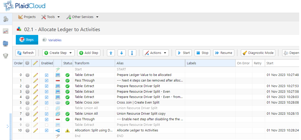
From here, you can manage Workflow Steps including creating or modifying existing workflow steps, changing the order, executing steps, and so on.
# Integrations
> Connect PlaidCloud to AI coding agents, PySpark, and other external tools your team already uses.
Connect PlaidCloud to the tools your team already uses.
[AI coding agents ](/integrations/ai-coding-agents/)Use Claude Code, Cursor, Copilot, ChatGPT, Gemini, and Claude Desktop with PlaidCloud's MCP server.
[PySpark ](/integrations/pyspark/)Run PySpark workloads against PlaidCloud data.
# AI Agents (MCP)
> Connect Claude, Cursor, GitHub Copilot, Gemini, and other AI agents to your PlaidCloud tenant through the Model Context Protocol (MCP) server.
PlaidCloud exposes a curated [Model Context Protocol](https://modelcontextprotocol.io) (MCP) server at `/mcp/` on every workspace. AI agents connect to it the same way they connect to any other MCP server, then call the tools to read projects, run workflows, query tables, manage dimensions, and more.
The pages in this section cover what the server exposes, how to authenticate, and step-by-step setup for the most common AI clients.
# ChatGPT
> Current state of MCP support in ChatGPT and recommended approaches for connecting ChatGPT to PlaidCloud.
ChatGPT’s support for user-added MCP servers is still rolling out and varies by plan tier and surface. This page describes what works today.
## Chatgpt Pro / Plus / Team — Connectors
[Section titled “Chatgpt Pro / Plus / Team — Connectors”](#chatgpt-pro--plus--team--connectors)
If your ChatGPT plan exposes the **Connectors** UI (Settings → Connectors), you can add PlaidCloud as a custom MCP connector:
1. Go to **Settings → Connectors → Add custom connector**.
2. Enter:
* **Name**: `PlaidCloud`
* **MCP server URL**: `https://.plaid.cloud/mcp/`
3. ChatGPT will redirect you to PlaidCloud for OAuth login. Approve the connection.
4. Toggle the connector on inside any conversation that should be able to use it.
Note
The Connectors UI may not be visible on every account or every region. If you don’t see “Add custom connector,” your plan or workspace policy doesn’t currently allow user-added MCP servers — use the workaround below.
## Chatgpt Enterprise
[Section titled “Chatgpt Enterprise”](#chatgpt-enterprise)
Enterprise admins can pin MCP connectors at the workspace level through the admin console. Follow the same OAuth setup as above but expect a workspace approval step from your admin before the connector becomes usable.
## Workaround — Custom Gpts With REST Actions
[Section titled “Workaround — Custom Gpts With REST Actions”](#workaround--custom-gpts-with-rest-actions)
If your account doesn’t support custom MCP connectors, you can still drive PlaidCloud from ChatGPT through a **Custom GPT** that calls PlaidCloud’s REST API as an OpenAPI Action:
1. PlaidCloud’s REST surface is described by the OpenAPI document at `https://.plaidcloud.org/openapi_rest.json`.
2. In ChatGPT, create a Custom GPT (Explore GPTs → Create) and under **Actions** import that URL (or paste the JSON).
3. Configure authentication as **OAuth** and point at PlaidCloud’s Keycloak endpoints. Your PlaidCloud admin can supply the realm URLs and client ID.
This trades MCP’s tool-name conventions for direct REST endpoints — slightly more verbose for the model to navigate, but functionally equivalent for the read/write operations PlaidCloud exposes.
## Why MCP Isn’t Always Available
[Section titled “Why MCP Isn’t Always Available”](#why-mcp-isnt-always-available)
OpenAI’s MCP support continues to evolve and the available surfaces (Connectors UI, Actions schema, etc.) change between plan tiers and over time. If the official **Connectors** path is open on your account, prefer it — it has built-in OAuth refresh and a tool-call experience matching the rest of this section. Falling back to Custom GPT Actions is only necessary when MCP isn’t yet exposed for your account.
# Claude Code
> Set up Claude Code (CLI, VSCode extension, JetBrains plugin) to call PlaidCloud's MCP tools using either OAuth or a static Bearer token.
[Claude Code](https://claude.com/claude-code) is Anthropic’s coding agent. It ships as a CLI, a VSCode extension, and a JetBrains plugin — all three share the same MCP configuration.
## Option a — OAuth (recommended)
[Section titled “Option a — OAuth (recommended)”](#option-a--oauth-recommended)
OAuth is the lowest-maintenance path. Claude Code’s MCP bridge handles the browser redirect and refresh transparently.
1. From your project root, add the server. The CLI form:
```bash
claude mcp add --transport http plaidcloud https://.plaid.cloud/mcp/
```
Or in `.mcp.json` at the project root:
```json
{
"mcpServers": {
"plaidcloud": {
"type": "http",
"url": "https://.plaid.cloud/mcp/"
}
}
}
```
2. Restart Claude Code. The first time you ask it to use a `plaidcloud_` tool, the bridge will pop up an authorization URL. Open it, sign in to PlaidCloud, approve the connection, and paste the callback URL Claude Code asked for. The token is cached locally and refreshed automatically.
3. Verify with `claude mcp list` (CLI) or `/mcp` (in-session). The server should show as connected.
Note
The OAuth bridge state can occasionally get stuck on remote/SSH sessions where Claude Code can’t reach `localhost` from your browser. If that happens, fall back to Option B.
## Option B — Static Bearer Token
[Section titled “Option B — Static Bearer Token”](#option-b--static-bearer-token)
When OAuth isn’t practical (remote sessions, devcontainers, agent runtimes that don’t survive browser redirects), use a Bearer token:
1. In a browser tab where you’re signed into PlaidCloud, open:
```plaintext
https://.plaid.cloud/mcp/setup/token
```
Click “Copy snippet.”
2. Paste it into your project’s `.mcp.json` under `mcpServers`:
```json
{
"mcpServers": {
"plaidcloud": {
"type": "http",
"url": "https://.plaid.cloud/mcp/",
"headers": {
"Authorization": "Bearer eyJhbGc…"
}
}
}
}
```
Or via the CLI:
```bash
claude mcp add --transport http plaidcloud \
https://.plaid.cloud/mcp/ \
-H "Authorization: Bearer eyJhbGc…"
```
3. Restart Claude Code. `claude mcp list` should show the server as connected.
When the token expires, reload the `/mcp/setup/token` URL and replace the `Authorization` value.
## Multi-Tenant Setup
[Section titled “Multi-Tenant Setup”](#multi-tenant-setup)
You can configure multiple PlaidCloud tenants side-by-side — give each a distinct name:
```json
{
"mcpServers": {
"plaidcloud-prod": { "type": "http", "url": "https://prod.plaid.cloud/mcp/" },
"plaidcloud-dev": { "type": "http", "url": "https://dev.plaid.cloud/mcp/" }
}
}
```
When you ask Claude Code to do something, name the tenant in your prompt (“in the dev tenant, find projects whose name starts with `Q4`”) so it picks the right server.
## Tips
[Section titled “Tips”](#tips)
* Run `mcp_introspect` early in a session so Claude Code understands the tool surface without re-reading the full manifest on every call.
* Mutating tools (`*_upsert`, `*_organize`, `*_run`) accept `dry_run=True` — useful when you’re letting an agent script changes and want a plan to review first.
* For long-running operations (workflow runs, query exports), prefer the `*_track` / `*_status` tools over poll loops — they’re the single source of truth and avoid flooding the agent’s context.
# Claude Desktop and Claude.ai
> Add PlaidCloud as a Custom Connector in Claude.ai (web) or Claude Desktop so the chat assistant can call MCP tools during conversations.
The consumer Claude app — both the web UI at [claude.ai](https://claude.ai) and the desktop app — supports MCP servers through its **Custom Connectors** feature. Setup is a one-time OAuth dance, after which the connection is associated with your Claude account and follows you across devices.
Note
Custom Connectors are available on Claude Pro, Max, Team, and Enterprise plans. Team and Enterprise admins can pin connectors for everyone in the workspace.
## Setup
[Section titled “Setup”](#setup)
1. In Claude (web or desktop), open **Settings → Connectors**.
2. Click **Add custom connector**.
3. Fill in:
* **Name**: `PlaidCloud` (or `PlaidCloud (prod)`, `PlaidCloud (dev)` if you have multiple tenants).
* **Server URL**: `https://.plaid.cloud/mcp/`
4. Click **Add**. Claude opens a browser tab to PlaidCloud’s Keycloak login.
5. Sign in and approve the connection. You’ll be redirected back to Claude with the connection saved.
The connector is now available in any conversation. Toggle it on (or off) using the connectors picker in the chat composer.
## Usage
[Section titled “Usage”](#usage)
Once enabled, you can ask Claude things like:
* “List the workflows in project `Q4 Forecast`.”
* “Show me the last 10 failed runs for the `daily-load` workflow.”
* “Run `mcp_recipes` and pick the right one for backfilling a step.”
Claude will pick the appropriate MCP tool, call it, and incorporate the response into its reply. For mutating operations it will typically narrate what it’s about to do — review carefully before approving.
## Multiple Tenants
[Section titled “Multiple Tenants”](#multiple-tenants)
Add a separate connector for each tenant. Give them distinct names so Claude can tell them apart in conversation. Only the connectors you toggle on for a given chat are available — leaving production off by default and only enabling it when you’re sure is a sensible safety habit.
## Refreshing Access
[Section titled “Refreshing Access”](#refreshing-access)
Custom connectors store an OAuth refresh token, so re-authentication is rare. If you change your PlaidCloud password, get a new device, or your session is invalidated server-side, the connector may show “needs authentication.” Click **Reconnect** in the connectors settings to redo the OAuth flow.
## Disconnecting
[Section titled “Disconnecting”](#disconnecting)
Settings → Connectors → click the connector → **Remove**. This deletes the OAuth tokens stored with your Claude account. The PlaidCloud-side session is independent — log out of PlaidCloud separately if you want to invalidate the underlying Keycloak session.
# GitHub Copilot
> Configure GitHub Copilot's agent mode in VSCode to use PlaidCloud's MCP tools.
GitHub Copilot’s [agent mode](https://docs.github.com/copilot/using-github-copilot/copilot-chat-in-ide/using-mcp-with-copilot) in VSCode supports MCP servers via a workspace or user-scoped `.vscode/mcp.json` (workspace) or the global VSCode `mcp.json` (user).
Note
Copilot’s MCP support is gated by Copilot plan tier and the `chat.mcp.enabled` setting in VSCode. Make sure both are enabled before configuring servers.
## Setup
[Section titled “Setup”](#setup)
1. Get a Bearer token by visiting `https://.plaid.cloud/mcp/setup/token` in a browser where you’re signed into PlaidCloud.
2. In VSCode, open the command palette and run **MCP: Add Server**, or create `.vscode/mcp.json` directly:
```json
{
"servers": {
"plaidcloud": {
"type": "http",
"url": "https://.plaid.cloud/mcp/",
"headers": {
"Authorization": "Bearer eyJhbGc…"
}
}
}
}
```
3. Reload VSCode. Open the Copilot chat panel, switch the mode dropdown to **Agent**, and confirm the PlaidCloud tools appear in the tools list (typically shown as `plaidcloud_*`).
## Usage
[Section titled “Usage”](#usage)
Ask Copilot to perform PlaidCloud operations directly:
* “Find all workflows in project `Q4 Forecast` whose last run failed.”
* “Show me the schema of table `customers` and suggest indexes.”
* “Run the `daily-load` workflow and report the run status.”
Copilot picks the appropriate tool, executes it, and quotes results in its reply. For destructive operations (delete, organize, upsert without `dry_run`), it will typically ask for confirmation — review the planned action before approving.
## Refreshing the Token
[Section titled “Refreshing the Token”](#refreshing-the-token)
VSCode reads `.vscode/mcp.json` on startup and on file change. When the token expires, reload `https://.plaid.cloud/mcp/setup/token` and overwrite the `Authorization` value — VSCode reloads the server automatically.
## Restricting to Specific Tools
[Section titled “Restricting to Specific Tools”](#restricting-to-specific-tools)
If you want to limit which PlaidCloud tools Copilot can call, use VSCode’s per-server tool allow-list (Settings → Copilot → MCP → server-specific tool selection). This is helpful for read-only sessions or for keeping mutating tools (`*_upsert`, `*_run`) gated behind explicit re-enable.
# Cursor
> Configure Cursor IDE to call PlaidCloud's MCP tools through its built-in MCP support.
[Cursor](https://cursor.com) supports MCP servers through a `mcp.json` config file. The shape is the same as Claude Code’s `.mcp.json`, so the same Bearer-token snippet works in both.
## Setup
[Section titled “Setup”](#setup)
1. Get a Bearer token by visiting `https://.plaid.cloud/mcp/setup/token` in a browser where you’re signed into PlaidCloud.
2. Open Cursor’s MCP config:
* **Project-scoped**: create `.cursor/mcp.json` in your project root.
* **User-scoped (all projects)**: create `~/.cursor/mcp.json` in your home directory.
3. Add the PlaidCloud server:
```json
{
"mcpServers": {
"plaidcloud": {
"url": "https://.plaid.cloud/mcp/",
"headers": {
"Authorization": "Bearer eyJhbGc…"
}
}
}
}
```
4. Open Cursor’s **Settings → MCP** to verify the server is connected. If it shows an error, see [Troubleshooting](../troubleshooting/).
## Using the Tools
[Section titled “Using the Tools”](#using-the-tools)
In Cursor’s Composer or chat panel, you can prompt the agent in plain English (“describe the structure of project `Q4 Forecast`”) and it will pick the appropriate `plaidcloud_*` tool. Tool calls and responses appear inline — review mutating operations before approving.
## Refreshing the Token
[Section titled “Refreshing the Token”](#refreshing-the-token)
When the token expires, reload `https://.plaid.cloud/mcp/setup/token` and paste the new value into `mcp.json`. Cursor picks up the change without a full restart — toggle the server off/on in **Settings → MCP** if needed.
## Multiple Tenants
[Section titled “Multiple Tenants”](#multiple-tenants)
Repeat the entry under a different name:
```json
{
"mcpServers": {
"plaidcloud-prod": { "url": "https://prod.plaid.cloud/mcp/", "headers": { "Authorization": "Bearer …" } },
"plaidcloud-dev": { "url": "https://dev.plaid.cloud/mcp/", "headers": { "Authorization": "Bearer …" } }
}
}
```
# Google Gemini CLI
> Configure Google's gemini-cli to call PlaidCloud's MCP tools.
Google’s [`gemini-cli`](https://github.com/google-gemini/gemini-cli) supports MCP servers through `~/.gemini/settings.json` (user-scoped) or `.gemini/settings.json` in a project root (project-scoped).
## Setup
[Section titled “Setup”](#setup)
1. Get a Bearer token by visiting `https://.plaid.cloud/mcp/setup/token` in a browser where you’re signed into PlaidCloud.
2. Edit `~/.gemini/settings.json` (create it if it doesn’t exist):
```json
{
"mcpServers": {
"plaidcloud": {
"httpUrl": "https://.plaid.cloud/mcp/",
"headers": {
"Authorization": "Bearer eyJhbGc…"
}
}
}
}
```
3. Restart `gemini`. Inside a session, run `/mcp` to verify the server is connected and list its tools.
## Usage
[Section titled “Usage”](#usage)
Prompt Gemini to use the PlaidCloud tools directly:
* “Use plaidcloud to list workflows in the `Sales Forecasting` project.”
* “Describe the columns of the `customers` table and the most recent snapshot.”
You can also call tools explicitly with the `/tools` command if you want to inspect a specific tool’s input schema before invoking it.
## Refreshing the Token
[Section titled “Refreshing the Token”](#refreshing-the-token)
When the token expires, reload `https://.plaid.cloud/mcp/setup/token` and update the `Authorization` value in `settings.json`. Restart `gemini` to pick up the change.
## Gemini Code Assist (IDE)
[Section titled “Gemini Code Assist (IDE)”](#gemini-code-assist-ide)
Gemini Code Assist in VSCode/JetBrains accepts the same `mcpServers` config under its agent settings. The schema matches the CLI form — paste the same snippet under the IDE’s MCP server settings panel.
# Getting Started with AI Coding Agents
> Overview of the PlaidCloud MCP server — what it exposes, authentication options, and the basics every AI agent client needs.
## What is the MCP Server?
[Section titled “What is the MCP Server?”](#what-is-the-mcp-server)
The [Model Context Protocol](https://modelcontextprotocol.io) is an open standard for letting AI agents talk to external tools and data. PlaidCloud runs an MCP server on every workspace that wraps the same core helpers the REST API uses — grouped by intent (`find`, `describe`, `upsert`, `run`, `organize`) so an agent can navigate the surface without loading 1,000+ low-level RPC method names.
The server lives at:
```text
https://.plaid.cloud/mcp/
```
Replace `` with your workspace subdomain (whatever you use to log into the PlaidCloud UI).
## What It Exposes
[Section titled “What It Exposes”](#what-it-exposes)
The catalog covers most of the day-to-day surface an agent needs:
* **Projects, workflows, steps** — find/describe/upsert/run/organize, including step-level rerun and version history.
* **Tables, views, queries** — schema introspection, query execution, exports, snapshots, branches.
* **Dimensions** — describe, find, upsert, version, manage nodes/aliases/properties.
* **Connections** — find/upsert/test connections to external systems.
* **Lakehouse** — branches, snapshots, optimize/vacuum operations.
* **Identity** — members, groups, sessions, distros.
* **Documents, dashboards, UDFs, editors, agents, publishes** — domain-specific tools.
* **Alteryx migration** — convert Alteryx workflows staged in Document and coordinate portfolio migration work.
* **Workflow logs and run tracking** — `workflow_logs`, `workflow_run_status`, `workflow_job_track`.
Every tool returns a uniform envelope `{ok, data, next_cursor?, total?}`; failures use `{ok: false, error: {code, retryable, message, hint?}}`. Mutations accept `dry_run=True` for plan-without-write validation.
For the live catalog, point your agent at the server and call `mcp_introspect` (no arguments) — that returns the current tool count, per-domain summaries, and parameter signatures. Use `mcp_recipes` for common multi-tool playbooks (paginating large lists, snapshot-then-modify, rerun a failed step, etc.).
## Authentication
[Section titled “Authentication”](#authentication)
PlaidCloud’s MCP server accepts two authentication paths:
1. **OAuth 2.1 + PKCE via Dynamic Client Registration (DCR).** This is what Claude.ai’s custom-connector UI uses, and it’s also the default for Claude Code’s MCP bridge. The client registers itself, redirects you to PlaidCloud’s Keycloak login, and gets back a token transparently. You don’t need to do anything other than pick “OAuth” in the client and approve the login.
2. **Static Bearer token in an `Authorization` header.** For agent runtimes that don’t have a usable browser redirect or that want a long-lived token in a config file. PlaidCloud exposes a helper page to mint one for you (see below).
### Getting a Static Bearer Token
[Section titled “Getting a Static Bearer Token”](#getting-a-static-bearer-token)
Open this URL in a browser tab where you’re already signed into PlaidCloud:
```text
https://.plaid.cloud/mcp/setup/token
```
The page returns a JSON snippet ready to paste into your agent’s MCP config. Each workspace has its own snippet.
The token’s lifespan is governed by your Keycloak realm’s access-token-lifespan policy (typically a few hours to a day). To refresh, reload the same URL — your browser session re-mints the token automatically.
Note
This flow is intended for getting started and for clients that can’t complete an OAuth redirect. For long-lived agent access in production — service accounts, CI runners, scheduled jobs — use OAuth where the client supports it. Personal Access Tokens are planned but not yet generally available.
## Pick a Client
[Section titled “Pick a Client”](#pick-a-client)
The rest of this section walks through setup for specific AI agent clients:
* [Claude Code](../claude-code/) — Anthropic’s coding agent (CLI, VSCode extension, JetBrains plugin).
* [Claude Desktop and Claude.ai](../claude-desktop/) — the consumer Claude app (desktop) and web (`claude.ai`) using “Custom Connectors.”
* [Cursor](../cursor/) — the AI-native code editor.
* [GitHub Copilot](../copilot/) — Copilot agent mode in VSCode.
* [Google Gemini CLI](../gemini/) — `gemini-cli` and Gemini Code Assist.
* [ChatGPT](../chatgpt/) — current support status and recommended workaround.
* [Troubleshooting](../troubleshooting/) — common errors and how to fix them.
# Troubleshooting
> Common issues connecting AI agents to the PlaidCloud MCP server and how to fix them.
## “failed to Connect” / “session Not Found”
[Section titled ““failed to Connect” / “session Not Found””](#failed-to-connect--session-not-found)
Symptom: the client config looks correct but the server shows as failed in the client’s MCP status panel. Server logs show 404 `Session not found` errors.
Cause: a known bug in some MCP clients (most notably Claude Code 2.1.111 with static `Authorization` headers) where the client doesn’t preserve `mcp-session-id` between successive HTTP requests. PlaidCloud’s MCP server runs in stateless HTTP mode to sidestep this — if you’re seeing it on a tenant that hasn’t been redeployed since the fix, ask your administrator to redeploy.
Until the redeploy lands, the OAuth flow (without static `Authorization` headers) still works because it uses a different code path in the client.
## ”oauth Flow is Not in Progress” During Claude Code Login
[Section titled “”oauth Flow is Not in Progress” During Claude Code Login”](#oauth-flow-is-not-in-progress-during-claude-code-login)
Symptom: you authorize in the browser, paste the callback URL into Claude Code, and it says no flow is in progress.
Cause: the bridge’s in-memory OAuth state is per-port and can be lost between the `authenticate` and `complete_authentication` tool calls — particularly in remote/SSH sessions where the browser callback can’t reach `localhost`.
Fix: switch to the static Bearer flow. Open `https://.plaid.cloud/mcp/setup/token` in a browser where you’re signed into PlaidCloud, copy the snippet into your `.mcp.json`, and restart Claude Code.
## Token Expired
[Section titled “Token Expired”](#token-expired)
Symptom: tools that worked yesterday now return 401 Unauthorized.
Cause: static Bearer tokens follow your Keycloak realm’s access-token-lifespan policy (typically a few hours to a day).
Fix: reload `https://.plaid.cloud/mcp/setup/token` to mint a fresh token, paste it into your config. For long-lived sessions, prefer OAuth — clients that support it refresh tokens automatically.
## ”no `access_token` in Session”
[Section titled “”no access\_token in Session””](#no-access_token-in-session)
Symptom: opening `/mcp/setup/token` shows “Sign-in required” or “No access\_token in session” even though you’re signed into PlaidCloud.
Cause: your session was established through a sign-in path that didn’t cache the Keycloak token (uncommon but possible).
Fix: sign out of PlaidCloud and sign back in through the standard login page. The new session will carry the access token.
## Tools Missing or Incomplete Catalog
[Section titled “Tools Missing or Incomplete Catalog”](#tools-missing-or-incomplete-catalog)
Symptom: `mcp_introspect` returns fewer tools than expected, or specific tools you need aren’t there.
Cause 1 — scopes: tools require specific PlaidCloud scopes (e.g. `analyze.workflow.write`). If your account lacks the scope, the tool will refuse to execute. Run `mcp_introspect(name='')` to see `required_scopes`. Ask your workspace admin to grant the scope or run the operation through an account that has it.
Cause 2 — version mismatch: an older deployment may not have all the tools described in the latest docs. Compare `mcp_introspect()`’s tool count to your current version’s release notes; ask for a redeploy if needed.
## Multi-Tenant: Which Tenant Did the Agent Just Hit?
[Section titled “Multi-Tenant: Which Tenant Did the Agent Just Hit?”](#multi-tenant-which-tenant-did-the-agent-just-hit)
Symptom: you have multiple PlaidCloud tenants configured and the agent’s response could’ve come from any of them.
Fix: include the tenant explicitly in your prompt (“in the **dev** tenant, list workflows…”). The MCP server names you chose in your config (e.g. `plaidcloud-prod`, `plaidcloud-dev`) double as identifiers the model can disambiguate against. For high-stakes operations, keep production toggled off in the connectors picker until you actively need it.
## Rate Limits and Quota
[Section titled “Rate Limits and Quota”](#rate-limits-and-quota)
PlaidCloud’s REST surface is rate-limited per requests-per-minute via the same middleware that fronts the UI. MCP calls share that limit. If an agent fires off a long burst of `find` calls (e.g. trying to enumerate every project + workflow + step), you may hit the limit. Use pagination (`cursor`, `limit`) and `count_only=True` for sizing checks instead of fetching the full result set.
## Getting Help
[Section titled “Getting Help”](#getting-help)
For server-side issues — auth failures, tools returning errors with no obvious cause, missing tools — check the response’s `error` envelope first. Every failure includes `code`, `retryable`, `message`, and often a `hint`. If the hint isn’t enough, contact your PlaidCloud administrator or open a support ticket with the request ID (returned in the `X-Request-Id` response header).
# PySpark and Spark Compute Clusters
> Build and run PySpark applications on PlaidCloud Spark compute clusters for distributed large-scale data analysis and processing.
Use PySpark with PlaidCloud — connect to project tables, read data into Spark DataFrames, and run distributed transformations alongside the rest of your data pipeline.
# Getting Started with PySpark
> Get started using PySpark in PlaidCloud for distributed data processing within user-defined functions and Jupyter Notebooks.
## PySpark Documentation
[Section titled “PySpark Documentation”](#pyspark-documentation)
PySpark is similar to using Pandas but allows for distributed compute and is not RAM bound. PySpark is available in both UDFs and Jupyter Notebooks.
## Spark Cluster
[Section titled “Spark Cluster”](#spark-cluster)
By default, workspaces do not have the Spark cluster enabled. To activate the Spark Cluster, go to the Workspace management app and enable the “Spark Compute Cluster” service.
Once activated, Spark jobs can be submitted to the cluster.
The cluster can be monitored from the `spark` sub-domain for the Workspace (e.g. `https://spark.my_workspace.plaid.cloud`)
# Reference
> Look up workflow steps, expressions, connectors, and CLI commands.
Reference material — search-driven rather than browse-driven. Use the search bar (⌘K / Ctrl-K) to jump straight to a specific function, step, or connector.
[Workflow steps ](/reference/workflow-steps/)Every step type — import, export, table ops, allocations, notifications, document handling, SAP integrations, and more.
[Alteryx Conversion Matrix ](/reference/alteryx-conversion-matrix/)How Alteryx tools convert to PlaidCloud workflow steps, macros, variables, artifacts, and managed executors.
[Expressions ](/reference/expressions/)SQL functions for Lakehouse v1 and v2 — array, string, datetime, aggregate, window, geo, and others.
[Connectors ](/reference/connectors/)Provider-by-provider reference for databases, ERPs, REST APIs, cloud storage, and open table formats.
[CLI ](/reference/cli/)PlaidLink, PlaidXL, and Jupyter CLI command references.
[Glossary ](/reference/glossary/)Definitions for every PlaidCloud term used across the documentation.
# Alteryx Conversion Matrix
> Coverage reference for how PlaidCloud converts Alteryx tools into Advanced workflow steps, macros, typed variables, Document assets, and managed job executors.
PlaidCloud converts Alteryx workflows, apps, and macros into Advanced workflows. The importer maps each Alteryx object to a native workflow step, macro construct, controlled variable, Document-backed file operation, or managed job executor.
Coverage levels:
* **Fully Converts** - converted directly to native PlaidCloud DAG behavior.
* **Converts With Validation** - converted to PlaidCloud behavior and should be validated against expected outputs for option-level parity.
* **Converts To Executor** - converted to a managed PlaidCloud job executor for specialized processing.
* **Cloud-Native Equivalent** - converted to a useful PlaidCloud artifact or operation that preserves the business purpose in a cloud-native form.
* **Annotation Only** - retained as workflow context, layout, or pass-through behavior with no separate runtime operation.
| Alteryx Object | Coverage Level | PlaidCloud Operation | Notes |
| ------------------------ | ------------------------ | ------------------------------------------------------- | ---------------------------------------------------------------------------------- |
| Action | Fully Converts | Variable binding and conditional step configuration | Updates downstream settings from converted app inputs. |
| AlteryxSelect | Fully Converts | Select and schema projection step | Keeps selected, renamed, and reordered fields. |
| AppendFields | Fully Converts | Append fields transform | Appends fields from one stream to another. |
| AutoField | Converts With Validation | Auto field sizing transform | Preserves inferred field sizing intent; validate schema where precision matters. |
| BrowseV2 | Annotation Only | Browse or passthrough marker | Preserved for inspection without adding runtime work. |
| Buffer | Converts To Executor | Spatial executor | Creates buffered geometries with validation against spatial fixtures. |
| CheckBoxGroup | Fully Converts | Controlled workflow variable | Converts app check box choices to controlled user input. |
| Classification | Converts To Executor | Machine learning executor | Runs classification logic through managed ML execution. |
| Condition | Fully Converts | Step condition with warning or error action | Uses workflow step conditions to trigger warnings, errors, or branches. |
| ControlParam | Fully Converts | Macro control parameter | Maps to PlaidCloud macro parameter handling. |
| CreatePoints | Fully Converts | Geometry point creation transform | Creates point geometry from coordinate fields. |
| CrossTab | Fully Converts | Pivot or cross-tab transform | Converts rows to columns. |
| DataCleansePro | Converts With Validation | Data cleanse transform | Cleans whitespace, nulls, punctuation, and casing according to configured options. |
| Date | Fully Converts | Workflow variable date value | Emits ISO date values for downstream steps and conditions. |
| DateTime | Converts With Validation | Date and time transform | Converts date and time parsing or formatting logic. |
| DbFileInput | Fully Converts | Document-backed file input or data materializer | Loads source files from Document into workflow data. |
| DbFileOutput | Fully Converts | Document-backed file output or table write | Writes output data to Document or PlaidCloud tables. |
| Detour | Fully Converts | Conditional branch routing | Converts route selection to DAG conditions. |
| DetourEnd | Fully Converts | Conditional branch merge | Rejoins conditionally selected branches. |
| Directory | Fully Converts | Document directory listing | Lists files from a Document path. |
| Distance | Converts To Executor | Spatial distance executor | Computes distance using managed spatial processing. |
| Download | Converts To Executor | HTTP download executor | Downloads external data or artifacts. |
| DropDown | Fully Converts | Controlled workflow variable | Converts app drop-down choices to controlled user input. |
| DynamicInput | Converts With Validation | Dynamic Document input | Resolves file patterns or variable-driven inputs at runtime. |
| DynamicRename | Fully Converts | Dynamic rename transform | Renames fields using metadata or configured rules. |
| DynamicReplace | Converts With Validation | Dynamic replace transform | Applies replacement rules from a second data stream. |
| DynamicSelect | Fully Converts | Dynamic field selection transform | Selects fields by type, name, or rule. |
| Error | Fully Converts | Step condition with error action | Converts configured error behavior to PlaidCloud step conditions. |
| FileBrowse | Fully Converts | Controlled Document file variable | Lets users choose a file for a converted app run. |
| Filter | Fully Converts | Filter transform | Splits records by expression into true and false paths. |
| FindNearest | Converts To Executor | Spatial nearest-neighbor executor | Finds nearest spatial records with managed spatial processing. |
| Fit | Converts To Executor | Model training executor | Trains or fits model behavior through managed execution. |
| FolderBrowse | Fully Converts | Controlled Document folder variable | Lets users choose a folder for a converted app run. |
| Formula | Fully Converts | Formula transform | Converts field expressions to PlaidCloud expressions or SQL-backed logic. |
| FuzzyMatch | Converts To Executor | Fuzzy matching executor | Uses managed fuzzy matching for match keys, thresholds, and candidate review. |
| Generalize | Converts To Executor | Spatial generalization executor | Simplifies geometry while preserving the requested spatial intent. |
| HtmlBox | Cloud-Native Equivalent | Report text or HTML artifact | Preserves content in PlaidCloud report or artifact output. |
| ImageToText | Converts To Executor | OCR executor | Extracts text from images through managed OCR. |
| Insights | Cloud-Native Equivalent | PlaidCloud dashboard or artifact output | Creates a cloud-native review artifact for repeatable sharing and review. |
| Join | Fully Converts | Join transform | Produces joined, left-only, and right-only streams. |
| JoinMultiple | Fully Converts | Multi-join transform | Joins multiple input streams. |
| Label | Annotation Only | Canvas label | Preserved as workflow context. |
| LabelGroup | Annotation Only | Canvas label group | Preserved as workflow context. |
| Link | Annotation Only | Canvas link or annotation | Preserved as workflow context. |
| ListBox | Fully Converts | Controlled workflow variable | Converts app list selections to controlled user input. |
| MacroInput | Fully Converts | PlaidCloud macro input port | Maps directly to a PlaidCloud macro input step. |
| MacroOutput | Fully Converts | PlaidCloud macro output port | Maps directly to a PlaidCloud macro output step. |
| Map | Cloud-Native Equivalent | Map artifact or spatial visualization | Creates a PlaidCloud map artifact for cloud review and sharing. |
| MapInput | Converts With Validation | Spatial input materializer | Loads spatial input data into the converted workflow. |
| Message | Fully Converts | Step condition with warning or message action | Emits workflow warning, message, or error based on configured condition. |
| Modeling | Converts To Executor | Machine learning executor | Runs model-oriented processing through managed execution. |
| MultiFieldFormula | Converts With Validation | Multi-field formula transform | Applies a formula across selected fields. |
| MultiRowFormula | Converts With Validation | Window or row-aware formula transform | Converts row-relative logic to PlaidCloud window behavior where possible. |
| NumericUpDown | Fully Converts | Controlled numeric workflow variable | Converts app numeric input to a typed variable. |
| Overlay | Converts To Executor | Spatial overlay executor | Performs spatial overlay operations through managed spatial processing. |
| PDFInput | Converts To Executor | PDF extraction executor | Extracts text or tables from PDFs. |
| PlotlyCharting | Cloud-Native Equivalent | Chart artifact | Creates a PlaidCloud chart artifact from converted data. |
| PolyBuild | Converts To Executor | Spatial polygon build executor | Builds polygon geometry from spatial inputs. |
| PortfolioComposerImage | Cloud-Native Equivalent | Report image artifact | Places images into generated PlaidCloud report artifacts. |
| PortfolioComposerLayout | Cloud-Native Equivalent | Report layout artifact | Converts layout intent to PlaidCloud report generation. |
| PortfolioComposerRender | Cloud-Native Equivalent | Report render artifact | Renders report output as a PlaidCloud artifact. |
| PortfolioComposerTable | Cloud-Native Equivalent | Report table artifact | Converts report table content to PlaidCloud report output. |
| PortfolioComposerText | Cloud-Native Equivalent | Report text artifact | Converts report text content to PlaidCloud report output. |
| Predict | Converts To Executor | Prediction executor | Scores records using managed model execution. |
| RadioButtonGroup | Fully Converts | Controlled workflow variable | Converts app radio choices to controlled user input. |
| RecordID | Fully Converts | Row identifier transform | Adds a deterministic record identifier. |
| RegEx | Fully Converts | Regular expression transform | Parses, matches, or replaces text using configured expressions. |
| Regression | Converts To Executor | Regression executor | Runs regression modeling through managed execution. |
| ReportMap | Cloud-Native Equivalent | Map report artifact | Produces a cloud-native map/report artifact. |
| Sample | Fully Converts | Sample transform | Keeps configured records by count, percentage, or grouping rule. |
| Smooth | Converts To Executor | Spatial smoothing executor | Smooths geometry through managed spatial processing. |
| Sort | Fully Converts | Sort transform | Sorts records by configured fields and directions. |
| SpatialInfo | Converts With Validation | Spatial metadata transform | Extracts spatial metadata such as area, length, centroid, or bounds. |
| SpatialMatch | Converts To Executor | Spatial match executor | Matches records by spatial relationship. |
| SpatialProcess | Converts To Executor | Spatial processing executor | Runs spatial operations that require executor-backed geometry handling. |
| Summarize | Fully Converts | Aggregate transform | Groups and aggregates records. |
| Tab | Annotation Only | App tab grouping | Preserved as converted app structure where relevant. |
| Test | Fully Converts | Step condition with warning or error action | Converts test assertions to PlaidCloud conditions. |
| TextBox | Fully Converts | Controlled text workflow variable | Converts app text input to a typed variable. |
| TextInput | Fully Converts | Inline table input | Creates inline data for the workflow. |
| TextPreProcessing | Converts To Executor | NLP preprocessing executor | Performs text normalization and preprocessing. |
| TextToColumns | Fully Converts | Split columns transform | Splits text into fields or rows. |
| Tile | Converts With Validation | Tile or grouping transform | Assigns tile groups according to configured rules. |
| ToolContainer | Annotation Only | Canvas container | Preserved as visual workflow organization. |
| TopicModel | Converts To Executor | Topic modeling executor | Runs topic modeling through managed NLP execution. |
| TradeArea | Converts To Executor | Spatial trade area executor | Creates trade area geometry through managed spatial processing. |
| Transformation | Converts With Validation | Transform step | Converts configured transformation logic to PlaidCloud expressions or SQL. |
| Transpose | Fully Converts | Unpivot transform | Converts columns to rows. |
| Tree | Fully Converts | Controlled workflow variable | Converts app tree selection to controlled user input. |
| Union | Fully Converts | Union transform | Combines streams by name, position, or configured field rules. |
| Unique | Fully Converts | Unique and duplicate split transform | Separates first unique records from duplicates. |
| VisualLayout | Annotation Only | Canvas layout metadata | Preserved as design context. |
| WordCloud | Cloud-Native Equivalent | Text visualization artifact | Creates a PlaidCloud visualization artifact from text analysis output. |
| XMLParse | Converts With Validation | XML parse transform | Extracts XML fields into workflow data. |
| Missing plugin reference | Fully Converts | Macro invocation or generated placeholder when resolved | Imports known macro sources and maps macro calls to PlaidCloud macro steps. |
## Validation Notes
[Section titled “Validation Notes”](#validation-notes)
For production workflows, validate converted outputs against trusted Alteryx outputs. PlaidCloud validation focuses on schema, row count, and row values, and ignores row order unless the workflow explicitly depends on ordered data.
Specialized operations such as spatial processing, fuzzy matching, machine learning, OCR, NLP, and reporting may run through managed job executors. These routes keep the converted workflow cloud-native while covering capabilities that are not best expressed as a single SQL transform.
# CLI Tools
> Reference for PlaidCloud command-line tools — PlaidLink agent, PlaidXL Excel add-in, and the Jupyter CLI for notebook integration.
PlaidCloud provides three command-line and on-machine tools for working with workspaces outside the web UI:
## PlaidLink
[Section titled “PlaidLink”](#plaidlink)
[PlaidLink](/reference/cli/plaidlink/) is an agent that runs inside your network to bridge PlaidCloud workflows to firewall-protected resources — databases, file shares, and other systems that PlaidCloud can’t reach directly. It installs as a Windows service, Unix/Linux/Mac daemon, container, or Kubernetes pod.
* [Install](/reference/cli/plaidlink/install/)
* [Configure](/reference/cli/plaidlink/configure/)
* [Agents](/reference/cli/plaidlink/agents/)
* [Upgrade](/reference/cli/plaidlink/upgrade/)
## PlaidXL
[Section titled “PlaidXL”](#plaidxl)
[PlaidXL](/reference/cli/plaidxl/) is the PlaidCloud Excel add-in. It lets analysts pull data from project tables, refresh saved queries, and read PlaidCloud variables directly inside Microsoft Excel.
* [Install](/reference/cli/plaidxl/install/)
* [Connect](/reference/cli/plaidxl/connect/)
* [Retrieve data](/reference/cli/plaidxl/retrieve/)
## Jupyter CLI
[Section titled “Jupyter CLI”](#jupyter-cli)
[Jupyter CLI](/reference/cli/jupyter/) lets data scientists work with PlaidCloud project data from Jupyter notebooks using a PlaidCloud-aware CLI and Python helpers.
* [Command line](/reference/cli/jupyter/command-line/)
* [Jupyter notebook](/reference/cli/jupyter/jupyter-notebook/)
* [OAuth setup](/reference/cli/jupyter/oauth-setup/)
# Jupyter Notebooks and Command Line Interfaces
> Access PlaidCloud directly through Jupyter Notebooks, command line interfaces, and API connections using OAuth token authentication.
PlaidCloud’s Jupyter integration lets data scientists work with project tables, run queries, and use PlaidCloud as a backing store from notebook environments. Authentication uses OAuth tokens so the same credentials work across the CLI, notebooks, and the REST API.
## Topics
[Section titled “Topics”](#topics)
* [Command line](/reference/cli/jupyter/command-line/) — the standalone CLI for scripted interactions
* [Jupyter notebook](/reference/cli/jupyter/jupyter-notebook/) — using PlaidCloud from notebook cells
* [OAuth setup](/reference/cli/jupyter/oauth-setup/) — wiring up authentication
# Command Line
> Use the PlaidCloud command line interface to automate tasks, run scripts, and interact with PlaidCloud resources via terminal.
PlaidCloud uses standard JSON-RPC requests and can be used with any application that can perform those requests.
To make things easier, a Python package is available to simplify the connection and API running process.
## Required Installation
[Section titled “Required Installation”](#required-installation)
From a terminal run the following command:
```bash
pip install plaidcloud-rpc
```
## Using the Simplerpc Object to Make a Request
[Section titled “Using the Simplerpc Object to Make a Request”](#using-the-simplerpc-object-to-make-a-request)
To make a request using the `plaidcloud-rpc` package use the `SimpleRPC` object.
```python
from plaidcloud.rpc.connection.jsonrpc import SimpleRPC
auth_token = "Your PlaidCloud Auth Token" # See Obtaining Token below
endpoint_uri = "plaidcloud.com" # or plaidcloud.net
rpc = SimpleRPC(auth_token, endpoint_uri)
```
Once you have the `SimpleRPC` object instantiated you can then issue RPC request to PlaidCloud. This example requests the meta data for a table.
```python
table = rpc.analyze.table.table(
project_id=project_id,
table_id=table_id
)
```
## What Apis Are Available?
[Section titled “What Apis Are Available?”](#what-apis-are-available)
There are many APIs available for use that control nearly every aspect of PlaidCloud. The interactive API reference is served per-tenant inside each PlaidCloud workspace — open your workspace and navigate to the API documentation menu to see the live endpoint catalog.
## Obtaining an OAuth Token
[Section titled “Obtaining an OAuth Token”](#obtaining-an-oauth-token)
See [OAuth setup](/reference/cli/jupyter/oauth-setup/) for more information on obtaining an OAuth token and how to configure the system for automated auth.
# Jupyter Notebooks
> Run Jupyter Notebooks in PlaidCloud for interactive data analysis, visualization, and Python-based data exploration workflows.
Jupyter Notebooks and Jupyter Lab provide exceptional interactive capabilities to analyze, explore, explain, and report data. PlaidCloud enables use of information directly in notebooks.
PlaidCloud provides JupyterHub within each tenant workspace if is activated for use. The documentation below helps with setting up Jupyter separately on a desktop or seperate server.
## Install Jupyter Notebook
[Section titled “Install Jupyter Notebook”](#install-jupyter-notebook)
This assumes you have a working Jupyter Notebook installation.
### Installing a Stand-Alone Jupyter Notebook
[Section titled “Installing a Stand-Alone Jupyter Notebook”](#installing-a-stand-alone-jupyter-notebook)
For more information on installing a Jupyter Notebook locally you can reference [Jupyter’s installation documentation](https://jupyter.org/install).
### Add to vs Code
[Section titled “Add to vs Code”](#add-to-vs-code)
VS Code also provides an extension that allows you to run notebooks directly in VS Code. Install the extension from the [Visual Studio Marketplace](https://marketplace.visualstudio.com/items?itemName=ms-toolsai.jupyter)
## Install PlaidCloud Utilities
[Section titled “Install PlaidCloud Utilities”](#install-plaidcloud-utilities)
While PlaidCloud can be accessed using stand OAuth and JSON-RPC requests, it is recommended that you use our pre-built libraries for simplified access. In addition, the PlaidCloud utilities library includes handy data helpers for use with Pandas dataframes.
To install the PlaidCloud Utilities perform the following pip installs:
```bash
pip install plaidcloud-rpc@git+https://github.com/PlaidCloud/plaid-rpc.git@v1.4.0#egg=plaidcloud-rpc
```
```bash
pip install plaidcloud-utilities@git+https://github.com/PlaidCloud/plaid-utilities.git@v1.5.2#egg=plaidcloud-utilities
```
## Obtaining an OAuth Token
[Section titled “Obtaining an OAuth Token”](#obtaining-an-oauth-token)
See [OAuth setup](/reference/cli/jupyter/oauth-setup/) for more information on obtaining an OAuth token and how to configure the system for automated auth.
## Open Jupyter Notebook User Interface
[Section titled “Open Jupyter Notebook User Interface”](#open-jupyter-notebook-user-interface)
Launch your notebook server to get started.
Once you are signed into your Jupyter notebook server, create a new notebook from the UI.
This will open a blank notebook.
Create a connection to communicate with PlaidCloud through the API endpoints
```python
from plaidcloud.utilities.connect import PlaidConnection
conn = PlaidConnection()
```
Establish a local table object and then query it with the results automatically placed in a [Pandas](https://pandas.pydata.org/) dataframe.
```python
tbl_sf_cust_master = conn.get_table('Salesforce_Customer_Master') # This gets a table object
df_sf_cust_master = conn.get_data(tbl_sf_cust_master) # This retrieves all the data into a dataframe
```
With that same table object you can also write more advanced queries using standard SQLAlchemy syntax.
```python
df_sf_cust_master_w_sales = conn.get_data(
tbl_sf_cust_master.select().with_only_columns(
[tbl_sf_cust_master.c.Id, tbl_sf_cust_master.c.CurrencyIsoCode, tbl_sf_cust_master.c.SyDSalesRegion]
).where(
tbl_sf_cust_master.c.TotalSalesPast3Years > 0
)
)
```
# OAuth Tokens
> Set up OAuth tokens for PlaidCloud API access to authenticate Jupyter Notebooks, CLI tools, and custom application connections.
PlaidCloud uses standard JSON-RPC requests and can be used with any application that can perform those requests. Requests are secured using OAuth tokens.
## Obtaining an OAuth Token
[Section titled “Obtaining an OAuth Token”](#obtaining-an-oauth-token)
OAuth tokens are generated from the PlaidCloud app. To view the list of current OAuth tokens assigned to you and generate new ones, navigate to `Analyze > Tools > Registered Systems`.
Once there you can view any existing tokens or choose to create a new one.
## Download OAuth PlaidCloud Config File
[Section titled “Download OAuth PlaidCloud Config File”](#download-oauth-plaidcloud-config-file)
Select “Register a New System”.
Fill out the form and note the name you entered so you can find it in the list.
Once created, open the registered system record by clicking on the gear icon. This will display the configuration file text.
NOTE: Be sure to select the project you want to use this connection for from the drop down at the top. It will add the Project Unique Identifier to the configuration.
Copy this text into a plaid.conf file located on your system. Place this in the .plaid directory.
## Create a Config File Locally
[Section titled “Create a Config File Locally”](#create-a-config-file-locally)
Create a directory one level up from your notebook directory or from where you plan to use command line interaction. Name the directory `.plaid`.
Inside the `.plaid` directory, create a file called `plaid.conf` and paste the contents you copied above into the file. Save the file and this will no allow you to connect using the PlaidCloud utilities and rpc methods.
## Advanced Uses
[Section titled “Advanced Uses”](#advanced-uses)
While it is convenient to locate the `.plaid` folder near its usage point, it can actually be placed anywhere in the upstream directory tree. The initialization process will traverse up the directory tree until it finds the `.plaid` directory.
Locating the `.plaid` directory higher up may be useful if you have multiple operations that need access but cannot coexist in the same lower level directory structures.
## Optional Paths Specification
[Section titled “Optional Paths Specification”](#optional-paths-specification)
If you are using a local Jupyter Notebook installation or operating from command line, it is possible to export data, excel files, and other data as well as reading in local data to dataframes using the helper tools. To do this, a paths.yaml file is necessary.
In addition to the `plaid.conf` file, create a `paths.yaml` file. The `paths.yaml` should be a sibling to the `plaid.conf` file inside the `.plaid` directory. It should contain the following path information:
```yaml
paths:
PROJECT_ROOT: '{WORKING_USER}/Documents'
LOCAL_STORAGE: '{PROJECT_ROOT}/local_storage'
DEBUG: '{PROJECT_ROOT}/local_storage'
REPORTS: '{PROJECT_ROOT}/reports'
create: []
local: {}
```
# PlaidLink
> Install and configure PlaidLink agents for secure access to systems behind firewalls, enabling remote queries and file transfers.
PlaidLink provides indirect access to client systems and processes that are protected by firewalls or behind other restrictions that make direct connections from within PlaidCloud difficult. By using a PlaidCloud Agent installed within the isolated area, PlaidCloud can request the agent perform actions like running queries, downloading or uploading files, checking sensor conditions, interacting with SAP, and much more.
Since the agent initiates contact with PlaidCloud and communicates over standard HTTPS network protocols, it can normally operate with minimal setup. In addition, the agent can run as an unprivileged user to control access rights within a restricted environment.
## Topics
[Section titled “Topics”](#topics)
* [Install](/reference/cli/plaidlink/install/) — getting PlaidLink running on Windows, Linux, macOS, or in a container
* [Configure](/reference/cli/plaidlink/configure/) — connection settings, credentials, and runtime options
* [Agents](/reference/cli/plaidlink/agents/) — managing multiple agents and their capabilities
* [Upgrade](/reference/cli/plaidlink/upgrade/) — moving to a newer PlaidLink build
# PlaidLink Agents
> Manage PlaidLink agents in PlaidCloud including registration, monitoring, status checks, and handling multiple agent deployments.
## Description
[Section titled “Description”](#description)
Sometimes it’s necessary and desireable to access data or run processes from a remote system that does not allow external access. This is common in enterprise environments behind firewalls. PlaidCloud allows this ability by using PlaidLink, which enables remote systems access behind a firewall or where direct access from PlaidCloud is not desired.
PlaidLink uses an agent-based system. This means that an agent, the remote user, is installed on a system inside the firewall or other restricted area. The agent can then connect to PlaidCloud by using an outbound initiation process over a secure HTTPS websocket connection. It is as secure as any other encrypted web connection and usually does not require you to open non-standard ports. Before gaining access, the agent must identify itself by sending its agent identifier. From this, if the agent has a successful authentication process, the agent is granted access to the approved operations.
PlaidLink can be installed on Windows, Unix, and Linux systems and can run under low privilege users. On Windows systems, PlaidLink can operate as a Windows Service with full control from the Service panel. On linux or unix systems, it can run as a deamon process.
PlaidLink can also run as a stand-alone Docker container or as a Kubernetes pod.
## Managing Agents
[Section titled “Managing Agents”](#managing-agents)
**To manage agents:**
1. Open Analyze
2. Select “Tools”
3. Click “PlaidLink Agents”
This brings you to the **PlaidLink Agents Table** where you can view, modify, and obtain credentials for the list of available agents.
## Creating an Agent
[Section titled “Creating an Agent”](#creating-an-agent)
**To create an agent:**
1. Open Analyze
2. Select “Tools”
3. Click “PlaidLink Agents”
4. Click “Add PlaidLink Agent”
5. Complete the required fields
6. Click “Create”
7. Assign the agent to the necessary security groups to access resources needed to perform its job
8. Assign the agent to the necessary Document accounts to access documents needed to perform its job
Danger
For Steps 7 and 8 above, the PlaidLink Agent must be assigned to security groups and document accounts necessary for performing the jobs you expect the Agent to perform. Otherwise it will be denied access.
Note
Any information not present on the new agent form will be automatically generated.
## Obtaining Agent Credentials
[Section titled “Obtaining Agent Credentials”](#obtaining-agent-credentials)
To configure PlaidLink agents on the remote system, you must first obtain the agent’s identifying information in order to maintain security. This information includes both a public and a private key.
**To obtain these keys:**
1. Open Analyze
2. Select “Tools”
3. Click “PlaidLink Agents”
4. Click the edit icon
This will open a form where you can view the public and private key values.
## Regenerating Agent Credentials
[Section titled “Regenerating Agent Credentials”](#regenerating-agent-credentials)
It is a good idea to periodically regenerate the public and private keys and update the configuration of remote systems in order to maintain security.
**To regenerate the credentials:**
1. Open Analyze
2. Select “Tools”
3. Click “PlaidLink Agents”
4. Click the regenerate icon
Once the credentials have been regenerated, they can be obtained in the same way a new agent’s credentials are obtained (described above).
## Enabling and Disabling an Agent
[Section titled “Enabling and Disabling an Agent”](#enabling-and-disabling-an-agent)
**To disable an agent:**
1. Open Analyze
2. Select “Tools”
3. Click “PlaidLink Agents”
4. Uncheck the “Active” checkbox
Note
When an agent is not marked as active, remote systems will not be able to connect using those agent credentials
## Running Multiple Agents
[Section titled “Running Multiple Agents”](#running-multiple-agents)
PlaidLink is designed to allow operation of multiple agents using a single service installation. Such a streamlined installation system permits one install to handle agents from multiple workspaces and / or agents with different levels of permissions for task execution.
To enable multiple agents, you simply add the agent credentials to the PlaidLink configuration file.
## Running Multiple PlaidLink Services
[Section titled “Running Multiple PlaidLink Services”](#running-multiple-plaidlink-services)
Similar to running multiple agents within one PlaidLink service, it is also possible to run multiple PlaidLink services.
This is sometimes necessary depending on use of system based security or network access restrictions that prevent communication across network boundaries.
Note
It is normally better to run multiple agents under a single service rather multiple services on a single machine. However, depending on the use case it may be necessary to run multiple distinct services.
## Compute, Memory, and Disk Requirements
[Section titled “Compute, Memory, and Disk Requirements”](#compute-memory-and-disk-requirements)
The PlaidLink service is extremely lightweight and only needs minimal compute and memory to operate. When processing significant data volumes it may be necessary to increase compute resources and especially memory.
Normally, the agent will happily run with 5% of CPU and 200MB of memory. For intense data operations, it is recommended to allocate an entire CPU and at least 4GB of RAM. For dynamic resource allocation systems like Kubernetes, it is fine if the agent has access to burstable resources rather than reserved resources.
Disk space for the agent is minimal too. Agent operations utilize disk space as a data buffer when transferring large amounts of data. Typically, 8GB of space is fine for normal operations. For intense data operations it is recommended that you scale disk up according to the expected data volumes. There is no set amount because it depends on several factors including CPU speed, network speed, amount of data, etc… However, a good place to start is 20GB and adjust from there.
## Networking Requirements
[Section titled “Networking Requirements”](#networking-requirements)
The PlaidLink Agent is designed to operate with minimal configuration required. It does not require any special VPN or network configuration other than allowing standard HTTPS network traffic. Agents communicate over the same protocol as normal web browser based traffic.
The agent service always initiates communication with PlaidCloud so there is no need to configure ingress access in firewalls.
Note
Sometimes firewall rules block all access, even standard HTTPS traffic. If the agent reports it is unable to contact PlaidCloud on startup, you will need to work with your networking team to open port 443 for traffic.
# Configure
> Configure PlaidLink agent settings in PlaidCloud including connection parameters, security options, and communication preferences.
The PlaidLink Agent works in conjunction with the PlaidCloud service. The PlaidLink Agent provides the connection necessary to operate with systems not accessible directly such as databases and file systems. The agent performs a number of essential actions including:
* Reading and writing to databases
* Reading and writing files to network drives and servers
* Checking for sensor conditions
* Interacting with SAP ECC and SAP S/4HANA through Remote Function Calls (RFCs)
* Interacting with SAP Profitability and Cost Management (PCM)
* Sending messages and notifications to remote systems
## Create an Agent on PlaidCloud
[Section titled “Create an Agent on PlaidCloud”](#create-an-agent-on-plaidcloud)
PlaidLink Agent management takes place within the Analyze tab of PlaidCloud. The first step is to create a new PlaidLink Agent instance on PlaidCloud.
### To Create a New PlaidLink Agent
[Section titled “To Create a New PlaidLink Agent”](#to-create-a-new-plaidlink-agent)
1. Select the Analyze tab
2. Select the tools menu from the top
3. Click PlaidLink Agents
4. Create a new Agent with an appropriate name for the environment or server that it will be installed on for remote operations
### To View the Agent Public and Private Keys
[Section titled “To View the Agent Public and Private Keys”](#to-view-the-agent-public-and-private-keys)
1. Click on the edit icon to view the form
2. At the bottom of the form you will find the public and private keys that were randomly generated during the Agent creation process
Note
Remember these keys, as they will be used in the agent configuration on the remote server.
### To Randomly Generate New Keys
[Section titled “To Randomly Generate New Keys”](#to-randomly-generate-new-keys)
1. Click on the Regenerate icon for the Agent record
2. Once the keys are regenerated, don’t forget to update the agent configuration file with the new keys on the remote server.
Note
Retain the public and private keys for configuring the remote agent in the next step.
## Document Account Access
[Section titled “Document Account Access”](#document-account-access)
If the agent will need to have access to a Document account for uploading or downloading files, it must be granted permission to access the Document account.
### To Grant Account Access
[Section titled “To Grant Account Access”](#to-grant-account-access)
1. In the Document tab select Manage Accounts
2. Once the table of accounts appears, click on the agent icon for the account which the new Agent should have upload/download rights
3. Drag the new agent into the Assigned Agents column
4. Save the access control form.
Note
Agents can only upload and download files if the agent has been granted access to one or more Document accounts.
## Data Connection Access
[Section titled “Data Connection Access”](#data-connection-access)
If the agent will need to have access to a data connection such as a database, it must be granted permission to access the external data connection information.
### To Grant Connection Access
[Section titled “To Grant Connection Access”](#to-grant-connection-access)
1. In the Analyze tab select the Tools menu
2. Click External Data Connections
3. Once the table of data connections appears, click on the agent icon for the connection, which the new Agent should have usage rights
4. Drag the new agent into the Assigned Agents column and save the access control form.
Note
Agent data connection credentials are managed in the External Data Connections.
### Next Step: Installing PlaidLink (agent) on a Remote System
[Section titled “Next Step: Installing PlaidLink (agent) on a Remote System”](#next-step-installing-plaidlink-agent-on-a-remote-system)
Follow these [Installation Instructions](/reference/cli/plaidlink/install) to install PlaidLink on the remote system.
# Install PlaidLink
> Install the PlaidLink agent on your local network or server to enable secure data access between PlaidCloud and protected systems.
## Download the Agent
[Section titled “Download the Agent”](#download-the-agent)
Check the releases on [PlaidCloud.com](https://plaidcloud.com/) for **PlaidLink**
## Extract the Agent
[Section titled “Extract the Agent”](#extract-the-agent)
Extract the downloaded zip file to an install location of your choice. Generally, this location will be:
```bash
C:\Users\\src\plaidlink
```
## Create a Configuration File
[Section titled “Create a Configuration File”](#create-a-configuration-file)
Note
If you are upgrading from a past version of the agent, the configuration file is still valid, and this step can be skipped
Copy the `config-dist.yaml` file in the agent’s directory to `%ProgramData\plaidcloud\`, and rename this copy `config.yaml`
*(Edit this configuration with the values retrieved from PlaidCloud)*
## Install the Agent’s Service
[Section titled “Install the Agent’s Service”](#install-the-agents-service)
Run the `install_windows_service.bat` file in the agent’s install directory OR
From an administrator command prompt, navigate to the agent’s install directory and run:
```bash
.\PlaidLink.exe install
```
## Running the Agent
[Section titled “Running the Agent”](#running-the-agent)
Note
To install a Windows service, one must have administrative privileges
Type **`Services`** into Windows’ search bar and open the service manager. In the list of services, find **`PlaidCloud Agent`**.
Right-click the service and select **“Start”** to start the agent.
## Freezing Updates
[Section titled “Freezing Updates”](#freezing-updates)
If at any point you want to disable the agent’s auto-update feature, open the agent’s **‘yaml’** configuration file, and at the root level of the file, add a line that reads `freeze_updates: true`, and restart the agent’s service.
Caution
Disabiling auto-updates is not recommended long-term
# Upgrade
> Upgrade your PlaidLink agent to the latest version to access new features, security patches, and improved system compatibility.
A manual upgrade of PlaidLink may be necessary if the agent does not have sufficient privileges to update itself when new versions are released or a manual upgrade process is desired.
## Download the Agent
[Section titled “Download the Agent”](#download-the-agent)
Check the releases on [PlaidCloud.com](https://plaidcloud.com/) for **PlaidLink**
## Stop the Current Agent
[Section titled “Stop the Current Agent”](#stop-the-current-agent)
Type **`Services`** into Windows’ search bar and open the service manager. In the list of services, find **`PlaidCloud Agent`**.
Right click on the **`PlaidCloud Agent`** service and select *Stop*. Once the service successfully stops, continue on.
## Extract the Agent
[Section titled “Extract the Agent”](#extract-the-agent)
Navigate to the current location of the installed agent.
```bash
C:\Users\\src\
```
Rename the current installation folder so that it will no longer be referenced. For example `Plaidlink_Old_12122022`
Extract the downloaded zip file to an install it in this location. Generally, this location will be:
```bash
C:\Users\\src\plaidlink
```
## Start the Agent
[Section titled “Start the Agent”](#start-the-agent)
Return to the *Services* window. Right click on the **`PlaidCloud Agent`** service and select *Start*.
Type **`Services`** into Windows’ search bar and open the service manager. In the list of services, find **`PlaidCloud Agent`**.
Right-click the service and select **`Start`** to start the agent. Once the agent shows in the **`Running`** state, the agent is now operational again on the new version.
# PlaidXL
> Use the PlaidXL Excel Add-in to interact with PlaidCloud workspaces, projects, tables, and variables directly from Excel.
The PlaidCloud Office Add-in (PlaidXL) lets analysts work with PlaidCloud workspaces, projects, workflows, tables, views, and variables directly from Microsoft Excel. PlaidXL provides Excel functions for pulling PlaidCloud data into worksheets and refreshing it on demand — useful for analysts who do their primary modeling in Excel but want their inputs to come from authoritative PlaidCloud project tables rather than copy-paste.
## Topics
[Section titled “Topics”](#topics)
* [Install](/reference/cli/plaidxl/install/) — downloading and enabling the PlaidXL add-in
* [Connect](/reference/cli/plaidxl/connect/) — signing in and choosing a workspace
* [Retrieve data](/reference/cli/plaidxl/retrieve/) — pulling project table data into Excel cells
# Connecting
> Connect PlaidXL to your PlaidCloud workspace to start importing, exporting, and managing data directly from Microsoft Excel.
## For PlaidCloud Logins
[Section titled “For PlaidCloud Logins”](#for-plaidcloud-logins)
Connecting to PlaidCloud is much like your login to PlaidCloud directly. You will be asked for your email, password, and any multi-factor authentication code enabled. Fill this out as normal, and begin using PlaidXL!
## For Single Sign-on Logins
[Section titled “For Single Sign-on Logins”](#for-single-sign-on-logins)
If you normally use single sign-on to access PlaidCloud, the login process will be transparent for you as long as you are currently logged into your organization. If you are not logged in, you will be prompted to sign in.
# Install PlaidXL
> Install the PlaidXL Excel Add-in to connect Microsoft Excel directly to PlaidCloud for data retrieval and management operations.
## For Windows
[Section titled “For Windows”](#for-windows)
1. From the `Insert > Add-ins` menu in Microsoft Excel, type in `PlaidCloud` in the add-in search box
2. Select the PlaidCloud Office Add-in and install it
## For Mac
[Section titled “For Mac”](#for-mac)
1. From the `Insert > Store` menu in Microsoft Excel for Mac, type in `PlaidCloud` in the add-in search box
2. Select the PlaidCloud Office Add-in and install it
# Working with Data
> Retrieve PlaidCloud data tables and views directly into Microsoft Excel using PlaidXL for local analysis and reporting tasks.
## Retrieve Data
[Section titled “Retrieve Data”](#retrieve-data)
To retrieve data from PlaidCloud, select your desired project from the dropdown menu. Once a project is selected, a list of tables in that project will appear. Click on a table to select it, and click the `Retrieve Table` button to import the selected table into Excel. The table will be placed in a new worksheet, named after the table. For your convenience, the following will also happen when a table is retrieved:
* Column headers will be frozen
* Auto-filters will be enabled
* An offset-based named range will be generated to encompass the data
* This range’s name will be the same as the table’s name, prefixed with an underscore and with all spaces replaced by underscores
* For example, the range for a table named “Sample data” would be “\_Sample\_data”
## Save Data
[Section titled “Save Data”](#save-data)
If you make changes data in the spreadsheet and want to push these changes to the PlaidCloud table, simply press the `Save Table (OVERWRITE!)` button.
Danger
Be careful – as the warning suggests, this will overwrite the data in PlaidCloud with the data in your spreadsheet.
Since you can open multiple PlaidCloud tables in PlaidXL, bulk operations are in place for your convenience. The pull/push all active tables buttons will retrieve the latest versions of all tables active in excel, or upload all active tables back to PlaidCloud, respectively.
In addition, pulling all tables will also refresh any pivot tables that use data from a refreshed table.
# Data and Service Connectors
> Connect PlaidCloud to external data sources and services including databases, ERPs, REST APIs, cloud storage, and Git repositories.
PlaidCloud connects to external data sources and services through purpose-built connectors. Each connector handles the authentication, protocol, and data-shape specifics of one provider family.
## Categories
[Section titled “Categories”](#categories)
### Databases and Data Lakes
[Section titled “Databases and Data Lakes”](#databases-and-data-lakes)
Relational databases, cloud warehouses, query engines, and lakehouse formats.
* [Databases](/reference/connectors/databases/) — PostgreSQL, MySQL, SQL Server, Oracle, Snowflake, Redshift, BigQuery, Databricks, and 15+ more
* [Open Tables](/reference/connectors/open-tables/) — Apache Iceberg, Delta Lake, Hudi, Hive open table formats
### Cloud and SaaS Services
[Section titled “Cloud and SaaS Services”](#cloud-and-saas-services)
* [REST](/reference/connectors/rest/) — Salesforce, NetSuite, Workday, QuickBooks, Stripe, Dynamics, and more
* [ERP systems](/reference/connectors/erp/) — SAP ECC, S/4HANA, Oracle EBS/Fusion, Infor, JD Edwards
* [Cloud services](/reference/connectors/cloud-services/) — third-party data services
* [Google](/reference/connectors/google/) — BigQuery, Google Sheets
* [Collaboration](/reference/connectors/collaboration/) — Slack, Microsoft Teams
* [Singer Sources](/reference/connectors/singer-sources/) — 130+ Singer-tap sources: Stripe, GitHub, HubSpot, databases, and more
### Development and Source Control
[Section titled “Development and Source Control”](#development-and-source-control)
* [Git providers](/reference/connectors/git/) — GitHub, GitLab, Bitbucket, Azure Repos, CodeCommit
## Related
[Section titled “Related”](#related)
* [Connections guide](/guides/connections/) — task-oriented walkthrough for creating and managing connections
* [Workflow steps reference](/reference/workflow-steps/) — what to do with a connection once it’s configured
# Cloud Service Connections
> Connect PlaidCloud to cloud data services including Quandl for financial and economic data integration into your workflows.
Connectors for cloud-based data services that use proprietary or non-REST protocols. These don’t fit cleanly into the database or REST categories.
## Providers
[Section titled “Providers”](#providers)
* [Quandl](/reference/connectors/cloud-services/quandl/) — financial and economic data (NASDAQ Data Link)
# Quandl Connector
> Set up a Quandl cloud service connection in PlaidCloud to import financial, economic, and alternative data into your workflows.
## Connection Documentation
[Section titled “Connection Documentation”](#connection-documentation)
[Quandl is now Nasdaq Data Link. The documentation](https://docs.data.nasdaq.com/).
## Setup
[Section titled “Setup”](#setup)
This connector uses a vendor-specific authentication flow and is configured directly from the **Connections** screen in your workspace. The configuration fields shown depend on the credentials your tenant administrator has provisioned for the integration.
See the upstream [quandl documentation](https://docs.data.nasdaq.com/) for the latest setup specifics.
If you need help setting up this connector for your tenant, contact your account team — connector-specific credentials, environment URLs, and any required pre-provisioning typically need to be coordinated with PlaidCloud support.
# Team Collaboration Connections
> Connect PlaidCloud to collaboration platforms like Slack and Microsoft Teams for automated notifications and data sharing.
PlaidCloud connects to team chat platforms so workflows can send notifications, alerts, or status updates directly into channels your team is already watching. Most commonly used alongside the [Notify via Slack](/reference/workflow-steps/notifications/notify-via-slack/) and [Notify via Microsoft Teams](/reference/workflow-steps/notifications/notify-via-microsoft-teams/) workflow steps.
## Providers
[Section titled “Providers”](#providers)
* [Slack](/reference/connectors/collaboration/slack/)
* [Microsoft Teams](/reference/connectors/collaboration/teams/)
# Slack Connector
> Configure a Slack connection in PlaidCloud to enable automated workflow notifications and data alerts to Slack channels.
## Connection Documentation
[Section titled “Connection Documentation”](#connection-documentation)
[Slack Admin documentation](https://slack.com/help).
## Setup
[Section titled “Setup”](#setup)
This connector uses a vendor-specific authentication flow and is configured directly from the **Connections** screen in your workspace. The configuration fields shown depend on the credentials your tenant administrator has provisioned for the integration.
See the upstream [slack documentation](https://api.slack.com/) for the latest setup specifics.
If you need help setting up this connector for your tenant, contact your account team — connector-specific credentials, environment URLs, and any required pre-provisioning typically need to be coordinated with PlaidCloud support.
# Microsoft Teams Connector
> Set up a Microsoft Teams connection in PlaidCloud to enable automated workflow notifications and data alerts to Teams channels.
## Connection Documentation
[Section titled “Connection Documentation”](#connection-documentation)
[Microsoft Teams Admin documentation](https://learn.microsoft.com/en-us/microsoftteams/).
## Setup
[Section titled “Setup”](#setup)
This connector uses a vendor-specific authentication flow and is configured directly from the **Connections** screen in your workspace. The configuration fields shown depend on the credentials your tenant administrator has provisioned for the integration.
See the upstream [teams documentation](https://learn.microsoft.com/en-us/microsoftteams/) for the latest setup specifics.
If you need help setting up this connector for your tenant, contact your account team — connector-specific credentials, environment URLs, and any required pre-provisioning typically need to be coordinated with PlaidCloud support.
# Database and Data Lake Connections
> Database and Data Lake connections vary by service. Each connector has specific security and access requirements for PlaidCloud to connect.
PlaidCloud connects directly to databases, data lakes, query engines, and lakehouses. Connections can also route through a PlaidLink Agent when the target sits behind a firewall.
The terms *database*, *lakehouse*, *query engine*, and *data warehouse* describe different underlying technologies but all expose a SQL-style query interface — so we treat them as one category here.
## Relational Databases
[Section titled “Relational Databases”](#relational-databases)
* [PostgreSQL](/reference/connectors/databases/postgres/)
* [MySQL](/reference/connectors/databases/mysql/)
* [Microsoft SQL Server](/reference/connectors/databases/microsoft-sql-server/)
* [Oracle](/reference/connectors/databases/oracle/)
* [IBM DB2](/reference/connectors/databases/ibm-db2/)
* [Informix](/reference/connectors/databases/informix/)
## Cloud Data Warehouses
[Section titled “Cloud Data Warehouses”](#cloud-data-warehouses)
* [Snowflake](/reference/connectors/databases/snowflake/)
* [Amazon Redshift](/reference/connectors/databases/amazon-redshift/)
* [Amazon Athena](/reference/connectors/databases/amazon-athena/)
* [Azure Databricks](/reference/connectors/databases/azure-databricks/)
* [Microsoft Fabric](/reference/connectors/databases/microsoft-fabric/)
* [SAP HANA](/reference/connectors/databases/sap-hana/)
## Analytical Databases
[Section titled “Analytical Databases”](#analytical-databases)
* [Greenplum](/reference/connectors/databases/greenplum/)
* [Exasol](/reference/connectors/databases/exasol/)
* [Databend](/reference/connectors/databases/databend/) — Lakehouse v1 engine
* [StarRocks](/reference/connectors/databases/starrocks/) — Lakehouse v2 engine
* [Doris](/reference/connectors/databases/doris/)
* [PlaidCloud Lakehouse](/reference/connectors/databases/plaidcloud-lakehouse/)
## Query Engines
[Section titled “Query Engines”](#query-engines)
* [Presto](/reference/connectors/databases/presto/)
* [Trino](/reference/connectors/databases/trino/)
* [Apache Hive](/reference/connectors/databases/hive/)
* [Apache Spark](/reference/connectors/databases/spark/)
## Generic
[Section titled “Generic”](#generic)
* [ODBC](/reference/connectors/databases/odbc/) — connect to any database with an ODBC driver
# Amazon Athena
> Configure an Amazon Athena connection in PlaidCloud to run serverless queries against data stored in Amazon S3 buckets.
**Amazon Athena** is AWS’s serverless query engine over S3-hosted data, billed per-query. Use this connector to run Athena queries from PlaidCloud workflows — useful for joining S3 data lakes with PlaidCloud project tables. Authentication uses AWS access keys or IAM role assumption.
## Upstream Documentation
[Section titled “Upstream Documentation”](#upstream-documentation)
[Amazon Athena documentation](https://docs.aws.amazon.com/athena/).
## Configuration
[Section titled “Configuration”](#configuration)
These fields appear when creating or editing this connection. Required vs optional depends on the authentication options you enable.
### Identification
[Section titled “Identification”](#identification)
| Field | Type | Description |
| ------------ | ----------------- | ---------------------------------------------------------------------- |
| Name | Text | Display name for this connection. |
| Alias | Text (multi-line) | Optional alias or notes about the connection. |
| Is active | Toggle | Whether the connection is enabled. Disable to pause without deleting. |
| Db read only | Toggle | Restrict the connection to read-only operations. |
| Access type | Select | Read-only, write-only, or read-write access level for this connection. |
### Connection
[Section titled “Connection”](#connection)
| Field | Type | Description |
| ---------- | ------ | ---------------------------------------------- |
| Db host | Text | Hostname or IP address of the database server. |
| Db port | Number | Port number for the database connection. |
| Db catalog | Text | Database, catalog, or schema to connect to. |
### Authentication
[Section titled “Authentication”](#authentication)
| Field | Type | Description |
| ----------- | -------- | ------------------------------------------------------------- |
| Db user | Text | Username for database authentication. |
| Use sso | Toggle | Authenticate via single sign-on instead of username/password. |
| Db password | Password | Password for database authentication. |
### SSL / TLS
[Section titled “SSL / TLS”](#ssl--tls)
| Field | Type | Description |
| -------------------- | ----------------- | ----------------------------------------------------------------------- |
| Use ssl | Toggle | Encrypt the connection with SSL/TLS. |
| Ssl mode | Select | SSL verification mode (e.g., disable, require, verify-ca, verify-full). |
| Ssl auth client cert | Text (multi-line) | Client certificate (PEM) for mutual TLS authentication. |
| Ssl auth client key | Text (multi-line) | Client private key (PEM) for mutual TLS authentication. |
| Ssl auth root cert | Text (multi-line) | Root CA certificate (PEM) for verifying the server’s cert. |
| Ssl auth cert revoke | Text (multi-line) | Certificate revocation list, if your environment uses one. |
### SSH Tunnel
[Section titled “SSH Tunnel”](#ssh-tunnel)
| Field | Type | Description |
| --------------- | ----------------- | ----------------------------------------------------------------------- |
| Use ssh | Toggle | Tunnel the connection through an SSH bastion. |
| Ssh host | Text | SSH bastion hostname. |
| Ssh port | Number | SSH bastion port (default 22). |
| Ssh user | Text | SSH bastion username. |
| Ssh password | Password | SSH bastion password (if password auth is used). |
| Use ssh cert | Toggle | Authenticate to the SSH bastion with a private key instead of password. |
| Ssh private key | Text (multi-line) | SSH private key (PEM) for bastion authentication. |
| Ssh host key | Text (multi-line) | Expected SSH host key for bastion fingerprint verification. |
# Amazon Redshift
> Set up an Amazon Redshift database connection in PlaidCloud to query, import, and export data with your Redshift warehouse.
**Amazon Redshift** is AWS’s managed cloud data warehouse, designed for analytical workloads over large datasets. Use this connector to read and write Redshift tables from PlaidCloud workflows. The connector speaks the PostgreSQL wire protocol; authentication uses standard database credentials or IAM-backed temporary credentials.
## Upstream Documentation
[Section titled “Upstream Documentation”](#upstream-documentation)
See the [Amazon Redshift documentation](https://docs.aws.amazon.com/redshift/) for guides and reference material.
## Configuration
[Section titled “Configuration”](#configuration)
These fields appear when creating or editing this connection. Required vs optional depends on the authentication options you enable.
### Identification
[Section titled “Identification”](#identification)
| Field | Type | Description |
| ------------ | ----------------- | ---------------------------------------------------------------------- |
| Name | Text | Display name for this connection. |
| Alias | Text (multi-line) | Optional alias or notes about the connection. |
| Is active | Toggle | Whether the connection is enabled. Disable to pause without deleting. |
| Db read only | Toggle | Restrict the connection to read-only operations. |
| Access type | Select | Read-only, write-only, or read-write access level for this connection. |
### Connection
[Section titled “Connection”](#connection)
| Field | Type | Description |
| ---------- | ------ | ---------------------------------------------- |
| Db host | Text | Hostname or IP address of the database server. |
| Db port | Number | Port number for the database connection. |
| Db catalog | Text | Database, catalog, or schema to connect to. |
### Authentication
[Section titled “Authentication”](#authentication)
| Field | Type | Description |
| ----------- | -------- | ------------------------------------------------------------- |
| Db user | Text | Username for database authentication. |
| Use sso | Toggle | Authenticate via single sign-on instead of username/password. |
| Db password | Password | Password for database authentication. |
### SSL / TLS
[Section titled “SSL / TLS”](#ssl--tls)
| Field | Type | Description |
| -------------------- | ----------------- | ----------------------------------------------------------------------- |
| Use ssl | Toggle | Encrypt the connection with SSL/TLS. |
| Ssl mode | Select | SSL verification mode (e.g., disable, require, verify-ca, verify-full). |
| Ssl auth client cert | Text (multi-line) | Client certificate (PEM) for mutual TLS authentication. |
| Ssl auth client key | Text (multi-line) | Client private key (PEM) for mutual TLS authentication. |
| Ssl auth root cert | Text (multi-line) | Root CA certificate (PEM) for verifying the server’s cert. |
| Ssl auth cert revoke | Text (multi-line) | Certificate revocation list, if your environment uses one. |
### SSH Tunnel
[Section titled “SSH Tunnel”](#ssh-tunnel)
| Field | Type | Description |
| --------------- | ----------------- | ----------------------------------------------------------------------- |
| Use ssh | Toggle | Tunnel the connection through an SSH bastion. |
| Ssh host | Text | SSH bastion hostname. |
| Ssh port | Number | SSH bastion port (default 22). |
| Ssh user | Text | SSH bastion username. |
| Ssh password | Password | SSH bastion password (if password auth is used). |
| Use ssh cert | Toggle | Authenticate to the SSH bastion with a private key instead of password. |
| Ssh private key | Text (multi-line) | SSH private key (PEM) for bastion authentication. |
| Ssh host key | Text (multi-line) | Expected SSH host key for bastion fingerprint verification. |
# Azure Databricks
> Configure an Azure Databricks connection in PlaidCloud to integrate Spark-based analytics and lakehouse data into workflows.
**Azure Databricks** combines Apache Spark, Delta Lake, and a managed notebook environment on Microsoft Azure. Use this connector to read and write tables in a Databricks workspace from PlaidCloud workflows. Authentication uses a personal access token or service principal; the workspace URL and HTTP path identify the SQL warehouse to target.
## Upstream Documentation
[Section titled “Upstream Documentation”](#upstream-documentation)
[Azure Databricks documentation](https://learn.microsoft.com/en-us/azure/databricks/).
## Configuration
[Section titled “Configuration”](#configuration)
These fields appear when creating or editing this connection. Required vs optional depends on the authentication options you enable.
### Identification
[Section titled “Identification”](#identification)
| Field | Type | Description |
| ------------ | ----------------- | ---------------------------------------------------------------------- |
| Name | Text | Display name for this connection. |
| Alias | Text (multi-line) | Optional alias or notes about the connection. |
| Is active | Toggle | Whether the connection is enabled. Disable to pause without deleting. |
| Db read only | Toggle | Restrict the connection to read-only operations. |
| Access type | Select | Read-only, write-only, or read-write access level for this connection. |
### Connection
[Section titled “Connection”](#connection)
| Field | Type | Description |
| ---------- | ---- | ---------------------------------------------- |
| Db host | Text | Hostname or IP address of the database server. |
| Db catalog | Text | Database, catalog, or schema to connect to. |
| Db schema | Text | Schema name within the database. |
### Authentication
[Section titled “Authentication”](#authentication)
| Field | Type | Description |
| ----------- | -------- | ------------------------------------------------------------- |
| Db user | Text | Username for database authentication. |
| Use sso | Toggle | Authenticate via single sign-on instead of username/password. |
| Db password | Password | Password for database authentication. |
### SSL / TLS
[Section titled “SSL / TLS”](#ssl--tls)
| Field | Type | Description |
| -------------------- | ----------------- | ----------------------------------------------------------------------- |
| Use ssl | Toggle | Encrypt the connection with SSL/TLS. |
| Ssl mode | Select | SSL verification mode (e.g., disable, require, verify-ca, verify-full). |
| Ssl auth client cert | Text (multi-line) | Client certificate (PEM) for mutual TLS authentication. |
| Ssl auth client key | Text (multi-line) | Client private key (PEM) for mutual TLS authentication. |
| Ssl auth root cert | Text (multi-line) | Root CA certificate (PEM) for verifying the server’s cert. |
| Ssl auth cert revoke | Text (multi-line) | Certificate revocation list, if your environment uses one. |
### SSH Tunnel
[Section titled “SSH Tunnel”](#ssh-tunnel)
| Field | Type | Description |
| --------------- | ----------------- | ----------------------------------------------------------------------- |
| Use ssh | Toggle | Tunnel the connection through an SSH bastion. |
| Ssh host | Text | SSH bastion hostname. |
| Ssh port | Number | SSH bastion port (default 22). |
| Ssh user | Text | SSH bastion username. |
| Ssh password | Password | SSH bastion password (if password auth is used). |
| Use ssh cert | Toggle | Authenticate to the SSH bastion with a private key instead of password. |
| Ssh private key | Text (multi-line) | SSH private key (PEM) for bastion authentication. |
| Ssh host key | Text (multi-line) | Expected SSH host key for bastion fingerprint verification. |
### Other
[Section titled “Other”](#other)
| Field | Type | Description |
| --------- | ---- | ----------- |
| Http path | Text | — |
# Databend
> Set up a Databend database connection in PlaidCloud to run cloud-native analytical queries with cost-effective data storage.
**Databend** is the open-source SQL engine that powers PlaidCloud’s Lakehouse v1. Use this connector when you want to query a standalone Databend deployment — for in-product analytics, the lakehouse is reachable through PlaidCloud directly without needing this connector.
## Upstream Documentation
[Section titled “Upstream Documentation”](#upstream-documentation)
[Databend documentation](https://docs.databend.com/guides/).
## Configuration
[Section titled “Configuration”](#configuration)
These fields appear when creating or editing this connection. Required vs optional depends on the authentication options you enable.
### Identification
[Section titled “Identification”](#identification)
| Field | Type | Description |
| ------------ | ----------------- | ---------------------------------------------------------------------- |
| Name | Text | Display name for this connection. |
| Alias | Text (multi-line) | Optional alias or notes about the connection. |
| Is active | Toggle | Whether the connection is enabled. Disable to pause without deleting. |
| Db read only | Toggle | Restrict the connection to read-only operations. |
| Access type | Select | Read-only, write-only, or read-write access level for this connection. |
### Connection
[Section titled “Connection”](#connection)
| Field | Type | Description |
| ---------- | ------ | ---------------------------------------------- |
| Db host | Text | Hostname or IP address of the database server. |
| Db port | Number | Port number for the database connection. |
| Db catalog | Text | Database, catalog, or schema to connect to. |
### Authentication
[Section titled “Authentication”](#authentication)
| Field | Type | Description |
| ----------- | -------- | ------------------------------------------------------------- |
| Db user | Text | Username for database authentication. |
| Use sso | Toggle | Authenticate via single sign-on instead of username/password. |
| Db password | Password | Password for database authentication. |
### SSL / TLS
[Section titled “SSL / TLS”](#ssl--tls)
| Field | Type | Description |
| -------------------- | ----------------- | ----------------------------------------------------------------------- |
| Use ssl | Toggle | Encrypt the connection with SSL/TLS. |
| Ssl mode | Select | SSL verification mode (e.g., disable, require, verify-ca, verify-full). |
| Ssl auth client cert | Text (multi-line) | Client certificate (PEM) for mutual TLS authentication. |
| Ssl auth client key | Text (multi-line) | Client private key (PEM) for mutual TLS authentication. |
| Ssl auth root cert | Text (multi-line) | Root CA certificate (PEM) for verifying the server’s cert. |
| Ssl auth cert revoke | Text (multi-line) | Certificate revocation list, if your environment uses one. |
### SSH Tunnel
[Section titled “SSH Tunnel”](#ssh-tunnel)
| Field | Type | Description |
| --------------- | ----------------- | ----------------------------------------------------------------------- |
| Use ssh | Toggle | Tunnel the connection through an SSH bastion. |
| Ssh host | Text | SSH bastion hostname. |
| Ssh port | Number | SSH bastion port (default 22). |
| Ssh user | Text | SSH bastion username. |
| Ssh password | Password | SSH bastion password (if password auth is used). |
| Use ssh cert | Toggle | Authenticate to the SSH bastion with a private key instead of password. |
| Ssh private key | Text (multi-line) | SSH private key (PEM) for bastion authentication. |
| Ssh host key | Text (multi-line) | Expected SSH host key for bastion fingerprint verification. |
# Apache Doris
> Configure an Apache Doris database connection in PlaidCloud to run real-time analytical queries on large-scale data sets.
**Apache Doris** is the high-performance MPP analytical database that StarRocks forked from. Use this connector to query Doris deployments from PlaidCloud workflows. Connection uses the MySQL wire protocol with standard username/password authentication.
## Upstream Documentation
[Section titled “Upstream Documentation”](#upstream-documentation)
[Apache Doris documentation](https://doris.apache.org/docs/4.x/gettingStarted/what-is-apache-doris).
The [Apache Doris project homepage](https://doris.apache.org/).
## Setup
[Section titled “Setup”](#setup)
This connector uses a vendor-specific authentication flow and is configured directly from the **Connections** screen in your workspace. The configuration fields shown depend on the credentials your tenant administrator has provisioned for the integration.
See the upstream [doris documentation](https://doris.apache.org/docs/) for the latest setup specifics.
If you need help setting up this connector for your tenant, contact your account team — connector-specific credentials, environment URLs, and any required pre-provisioning typically need to be coordinated with PlaidCloud support.
# Exasol
> Configure an Exasol database connection in PlaidCloud to run high-performance analytical queries and integrate your data.
**Exasol** is an in-memory analytical database optimized for fast SQL over large datasets. Use this connector to read and write Exasol tables from PlaidCloud workflows. Connection uses standard username/password authentication with optional SSL.
## Upstream Documentation
[Section titled “Upstream Documentation”](#upstream-documentation)
[Exasol documentation](https://docs.exasol.com/home.htm).
## Configuration
[Section titled “Configuration”](#configuration)
These fields appear when creating or editing this connection. Required vs optional depends on the authentication options you enable.
### Identification
[Section titled “Identification”](#identification)
| Field | Type | Description |
| ------------ | ----------------- | ---------------------------------------------------------------------- |
| Name | Text | Display name for this connection. |
| Alias | Text (multi-line) | Optional alias or notes about the connection. |
| Is active | Toggle | Whether the connection is enabled. Disable to pause without deleting. |
| Db read only | Toggle | Restrict the connection to read-only operations. |
| Access type | Select | Read-only, write-only, or read-write access level for this connection. |
### Connection
[Section titled “Connection”](#connection)
| Field | Type | Description |
| ---------- | ------ | ---------------------------------------------- |
| Db host | Text | Hostname or IP address of the database server. |
| Db port | Number | Port number for the database connection. |
| Db catalog | Text | Database, catalog, or schema to connect to. |
### Authentication
[Section titled “Authentication”](#authentication)
| Field | Type | Description |
| ----------- | -------- | ------------------------------------------------------------- |
| Db user | Text | Username for database authentication. |
| Use sso | Toggle | Authenticate via single sign-on instead of username/password. |
| Db password | Password | Password for database authentication. |
### SSL / TLS
[Section titled “SSL / TLS”](#ssl--tls)
| Field | Type | Description |
| -------------------- | ----------------- | ----------------------------------------------------------------------- |
| Use ssl | Toggle | Encrypt the connection with SSL/TLS. |
| Ssl mode | Select | SSL verification mode (e.g., disable, require, verify-ca, verify-full). |
| Ssl auth client cert | Text (multi-line) | Client certificate (PEM) for mutual TLS authentication. |
| Ssl auth client key | Text (multi-line) | Client private key (PEM) for mutual TLS authentication. |
| Ssl auth root cert | Text (multi-line) | Root CA certificate (PEM) for verifying the server’s cert. |
| Ssl auth cert revoke | Text (multi-line) | Certificate revocation list, if your environment uses one. |
### SSH Tunnel
[Section titled “SSH Tunnel”](#ssh-tunnel)
| Field | Type | Description |
| --------------- | ----------------- | ----------------------------------------------------------------------- |
| Use ssh | Toggle | Tunnel the connection through an SSH bastion. |
| Ssh host | Text | SSH bastion hostname. |
| Ssh port | Number | SSH bastion port (default 22). |
| Ssh user | Text | SSH bastion username. |
| Ssh password | Password | SSH bastion password (if password auth is used). |
| Use ssh cert | Toggle | Authenticate to the SSH bastion with a private key instead of password. |
| Ssh private key | Text (multi-line) | SSH private key (PEM) for bastion authentication. |
| Ssh host key | Text (multi-line) | Expected SSH host key for bastion fingerprint verification. |
# Greenplum
> Set up a Greenplum database connection in PlaidCloud to query, import, and export data with your Greenplum data warehouse.
**Greenplum** is a massively parallel PostgreSQL-derived analytical database (originally Pivotal, now VMware Tanzu). Use this connector to read and write Greenplum tables from PlaidCloud workflows. The wire protocol is PostgreSQL-compatible, so most PostgreSQL tooling considerations apply.
## Upstream Documentation
[Section titled “Upstream Documentation”](#upstream-documentation)
[The Greenplum documentation](https://techdocs.broadcom.com/us/en/vmware-tanzu/data-solutions/tanzu-greenplum/7/greenplum-database/landing-index.html).
## Configuration
[Section titled “Configuration”](#configuration)
These fields appear when creating or editing this connection. Required vs optional depends on the authentication options you enable.
### Identification
[Section titled “Identification”](#identification)
| Field | Type | Description |
| ------------ | ----------------- | ---------------------------------------------------------------------- |
| Name | Text | Display name for this connection. |
| Alias | Text (multi-line) | Optional alias or notes about the connection. |
| Is active | Toggle | Whether the connection is enabled. Disable to pause without deleting. |
| Db read only | Toggle | Restrict the connection to read-only operations. |
| Access type | Select | Read-only, write-only, or read-write access level for this connection. |
### Connection
[Section titled “Connection”](#connection)
| Field | Type | Description |
| ---------- | ------ | ---------------------------------------------- |
| Db host | Text | Hostname or IP address of the database server. |
| Db port | Number | Port number for the database connection. |
| Db catalog | Text | Database, catalog, or schema to connect to. |
### Authentication
[Section titled “Authentication”](#authentication)
| Field | Type | Description |
| ----------- | -------- | ------------------------------------------------------------- |
| Db user | Text | Username for database authentication. |
| Use sso | Toggle | Authenticate via single sign-on instead of username/password. |
| Db password | Password | Password for database authentication. |
### SSL / TLS
[Section titled “SSL / TLS”](#ssl--tls)
| Field | Type | Description |
| -------------------- | ----------------- | ----------------------------------------------------------------------- |
| Use ssl | Toggle | Encrypt the connection with SSL/TLS. |
| Ssl mode | Select | SSL verification mode (e.g., disable, require, verify-ca, verify-full). |
| Ssl auth client cert | Text (multi-line) | Client certificate (PEM) for mutual TLS authentication. |
| Ssl auth client key | Text (multi-line) | Client private key (PEM) for mutual TLS authentication. |
| Ssl auth root cert | Text (multi-line) | Root CA certificate (PEM) for verifying the server’s cert. |
| Ssl auth cert revoke | Text (multi-line) | Certificate revocation list, if your environment uses one. |
### SSH Tunnel
[Section titled “SSH Tunnel”](#ssh-tunnel)
| Field | Type | Description |
| --------------- | ----------------- | ----------------------------------------------------------------------- |
| Use ssh | Toggle | Tunnel the connection through an SSH bastion. |
| Ssh host | Text | SSH bastion hostname. |
| Ssh port | Number | SSH bastion port (default 22). |
| Ssh user | Text | SSH bastion username. |
| Ssh password | Password | SSH bastion password (if password auth is used). |
| Use ssh cert | Toggle | Authenticate to the SSH bastion with a private key instead of password. |
| Ssh private key | Text (multi-line) | SSH private key (PEM) for bastion authentication. |
| Ssh host key | Text (multi-line) | Expected SSH host key for bastion fingerprint verification. |
# Apache Hive
> Set up an Apache Hive data lake connection in PlaidCloud to query and integrate large-scale data stored in Hadoop ecosystems.
**Apache Hive** is the SQL layer over Hadoop-style distributed storage, common in older data lake deployments. Use this connector to read and write Hive tables. Authentication varies by deployment — common modes are LDAP, Kerberos, or no-auth on internal networks; check your Hive metastore configuration.
## Upstream Documentation
[Section titled “Upstream Documentation”](#upstream-documentation)
[Apache Hive documentation](https://hive.apache.org/docs/latest/).
## Configuration
[Section titled “Configuration”](#configuration)
These fields appear when creating or editing this connection. Required vs optional depends on the authentication options you enable.
### Identification
[Section titled “Identification”](#identification)
| Field | Type | Description |
| ------------ | ----------------- | ---------------------------------------------------------------------- |
| Name | Text | Display name for this connection. |
| Alias | Text (multi-line) | Optional alias or notes about the connection. |
| Is active | Toggle | Whether the connection is enabled. Disable to pause without deleting. |
| Db read only | Toggle | Restrict the connection to read-only operations. |
| Access type | Select | Read-only, write-only, or read-write access level for this connection. |
### Connection
[Section titled “Connection”](#connection)
| Field | Type | Description |
| ---------- | ------ | ---------------------------------------------- |
| Db host | Text | Hostname or IP address of the database server. |
| Db port | Number | Port number for the database connection. |
| Db catalog | Text | Database, catalog, or schema to connect to. |
### Authentication
[Section titled “Authentication”](#authentication)
| Field | Type | Description |
| ----------- | -------- | ------------------------------------------------------------- |
| Db user | Text | Username for database authentication. |
| Use sso | Toggle | Authenticate via single sign-on instead of username/password. |
| Db password | Password | Password for database authentication. |
### SSL / TLS
[Section titled “SSL / TLS”](#ssl--tls)
| Field | Type | Description |
| -------------------- | ----------------- | ----------------------------------------------------------------------- |
| Use ssl | Toggle | Encrypt the connection with SSL/TLS. |
| Ssl mode | Select | SSL verification mode (e.g., disable, require, verify-ca, verify-full). |
| Ssl auth client cert | Text (multi-line) | Client certificate (PEM) for mutual TLS authentication. |
| Ssl auth client key | Text (multi-line) | Client private key (PEM) for mutual TLS authentication. |
| Ssl auth root cert | Text (multi-line) | Root CA certificate (PEM) for verifying the server’s cert. |
| Ssl auth cert revoke | Text (multi-line) | Certificate revocation list, if your environment uses one. |
### SSH Tunnel
[Section titled “SSH Tunnel”](#ssh-tunnel)
| Field | Type | Description |
| --------------- | ----------------- | ----------------------------------------------------------------------- |
| Use ssh | Toggle | Tunnel the connection through an SSH bastion. |
| Ssh host | Text | SSH bastion hostname. |
| Ssh port | Number | SSH bastion port (default 22). |
| Ssh user | Text | SSH bastion username. |
| Ssh password | Password | SSH bastion password (if password auth is used). |
| Use ssh cert | Toggle | Authenticate to the SSH bastion with a private key instead of password. |
| Ssh private key | Text (multi-line) | SSH private key (PEM) for bastion authentication. |
| Ssh host key | Text (multi-line) | Expected SSH host key for bastion fingerprint verification. |
# IBM DB2
> Configure an IBM DB2 database connection in PlaidCloud to query, import, and export data with your DB2 database instances.
**IBM DB2** is IBM’s enterprise database, common in mainframe and mid-range environments. Use this connector to read and write DB2 tables from PlaidCloud workflows. Network access to the DB2 listener is required; for mainframe deployments, an SSH or VPN tunnel is typically required.
## Upstream Documentation
[Section titled “Upstream Documentation”](#upstream-documentation)
[The IBM DB2 documentation](https://www.ibm.com/support/pages/db2-database-product-documentation).
## Configuration
[Section titled “Configuration”](#configuration)
These fields appear when creating or editing this connection. Required vs optional depends on the authentication options you enable.
### Identification
[Section titled “Identification”](#identification)
| Field | Type | Description |
| ------------ | ----------------- | ---------------------------------------------------------------------- |
| Name | Text | Display name for this connection. |
| Alias | Text (multi-line) | Optional alias or notes about the connection. |
| Is active | Toggle | Whether the connection is enabled. Disable to pause without deleting. |
| Db read only | Toggle | Restrict the connection to read-only operations. |
| Access type | Select | Read-only, write-only, or read-write access level for this connection. |
### Connection
[Section titled “Connection”](#connection)
| Field | Type | Description |
| ---------- | ------ | ---------------------------------------------- |
| Db host | Text | Hostname or IP address of the database server. |
| Db port | Number | Port number for the database connection. |
| Db catalog | Text | Database, catalog, or schema to connect to. |
### Authentication
[Section titled “Authentication”](#authentication)
| Field | Type | Description |
| ----------- | -------- | ------------------------------------------------------------- |
| Db user | Text | Username for database authentication. |
| Use sso | Toggle | Authenticate via single sign-on instead of username/password. |
| Db password | Password | Password for database authentication. |
### SSL / TLS
[Section titled “SSL / TLS”](#ssl--tls)
| Field | Type | Description |
| -------------------- | ----------------- | ----------------------------------------------------------------------- |
| Use ssl | Toggle | Encrypt the connection with SSL/TLS. |
| Ssl mode | Select | SSL verification mode (e.g., disable, require, verify-ca, verify-full). |
| Ssl auth client cert | Text (multi-line) | Client certificate (PEM) for mutual TLS authentication. |
| Ssl auth client key | Text (multi-line) | Client private key (PEM) for mutual TLS authentication. |
| Ssl auth root cert | Text (multi-line) | Root CA certificate (PEM) for verifying the server’s cert. |
| Ssl auth cert revoke | Text (multi-line) | Certificate revocation list, if your environment uses one. |
### SSH Tunnel
[Section titled “SSH Tunnel”](#ssh-tunnel)
| Field | Type | Description |
| --------------- | ----------------- | ----------------------------------------------------------------------- |
| Use ssh | Toggle | Tunnel the connection through an SSH bastion. |
| Ssh host | Text | SSH bastion hostname. |
| Ssh port | Number | SSH bastion port (default 22). |
| Ssh user | Text | SSH bastion username. |
| Ssh password | Password | SSH bastion password (if password auth is used). |
| Use ssh cert | Toggle | Authenticate to the SSH bastion with a private key instead of password. |
| Ssh private key | Text (multi-line) | SSH private key (PEM) for bastion authentication. |
| Ssh host key | Text (multi-line) | Expected SSH host key for bastion fingerprint verification. |
# IBM Informix
> Set up an IBM Informix database connection in PlaidCloud to query, import, and export data with your Informix instances.
**IBM Informix** is IBM’s transactional database, common in retail and OLTP deployments. Use this connector to read and write Informix tables from PlaidCloud workflows. Network access to the Informix server is required; SSH tunneling is supported for non-flat networks.
## Upstream Documentation
[Section titled “Upstream Documentation”](#upstream-documentation)
[IBM Informix documentation](https://www.ibm.com/docs/ar/informix-servers/14.10.0?).
## Configuration
[Section titled “Configuration”](#configuration)
These fields appear when creating or editing this connection. Required vs optional depends on the authentication options you enable.
### Identification
[Section titled “Identification”](#identification)
| Field | Type | Description |
| ------------ | ----------------- | ---------------------------------------------------------------------- |
| Name | Text | Display name for this connection. |
| Alias | Text (multi-line) | Optional alias or notes about the connection. |
| Is active | Toggle | Whether the connection is enabled. Disable to pause without deleting. |
| Db read only | Toggle | Restrict the connection to read-only operations. |
| Access type | Select | Read-only, write-only, or read-write access level for this connection. |
### Connection
[Section titled “Connection”](#connection)
| Field | Type | Description |
| ---------- | ------ | ---------------------------------------------- |
| Db host | Text | Hostname or IP address of the database server. |
| Db port | Number | Port number for the database connection. |
| Db catalog | Text | Database, catalog, or schema to connect to. |
### Authentication
[Section titled “Authentication”](#authentication)
| Field | Type | Description |
| ----------- | -------- | ------------------------------------------------------------- |
| Db user | Text | Username for database authentication. |
| Use sso | Toggle | Authenticate via single sign-on instead of username/password. |
| Db password | Password | Password for database authentication. |
### SSL / TLS
[Section titled “SSL / TLS”](#ssl--tls)
| Field | Type | Description |
| -------------------- | ----------------- | ----------------------------------------------------------------------- |
| Use ssl | Toggle | Encrypt the connection with SSL/TLS. |
| Ssl mode | Select | SSL verification mode (e.g., disable, require, verify-ca, verify-full). |
| Ssl auth client cert | Text (multi-line) | Client certificate (PEM) for mutual TLS authentication. |
| Ssl auth client key | Text (multi-line) | Client private key (PEM) for mutual TLS authentication. |
| Ssl auth root cert | Text (multi-line) | Root CA certificate (PEM) for verifying the server’s cert. |
| Ssl auth cert revoke | Text (multi-line) | Certificate revocation list, if your environment uses one. |
### SSH Tunnel
[Section titled “SSH Tunnel”](#ssh-tunnel)
| Field | Type | Description |
| --------------- | ----------------- | ----------------------------------------------------------------------- |
| Use ssh | Toggle | Tunnel the connection through an SSH bastion. |
| Ssh host | Text | SSH bastion hostname. |
| Ssh port | Number | SSH bastion port (default 22). |
| Ssh user | Text | SSH bastion username. |
| Ssh password | Password | SSH bastion password (if password auth is used). |
| Use ssh cert | Toggle | Authenticate to the SSH bastion with a private key instead of password. |
| Ssh private key | Text (multi-line) | SSH private key (PEM) for bastion authentication. |
| Ssh host key | Text (multi-line) | Expected SSH host key for bastion fingerprint verification. |
# Microsoft Fabric
> Configure a Microsoft Fabric connection in PlaidCloud to integrate analytics, data warehousing, and lakehouse capabilities.
**Microsoft Fabric** combines Power BI, Synapse, and Data Factory into a unified analytics platform. Use this connector to access Fabric warehouses and lakehouses as relational sources from PlaidCloud workflows. Authentication is through a SQL Server-compatible endpoint plus your Microsoft tenant credentials.
## Upstream Documentation
[Section titled “Upstream Documentation”](#upstream-documentation)
[The Microsoft Fabric documentation](https://learn.microsoft.com/en-us/fabric/).
## Configuration
[Section titled “Configuration”](#configuration)
These fields appear when creating or editing this connection. Required vs optional depends on the authentication options you enable.
### Identification
[Section titled “Identification”](#identification)
| Field | Type | Description |
| ------------ | ----------------- | ---------------------------------------------------------------------- |
| Name | Text | Display name for this connection. |
| Alias | Text (multi-line) | Optional alias or notes about the connection. |
| Is active | Toggle | Whether the connection is enabled. Disable to pause without deleting. |
| Db read only | Toggle | Restrict the connection to read-only operations. |
| Access type | Select | Read-only, write-only, or read-write access level for this connection. |
### Connection
[Section titled “Connection”](#connection)
| Field | Type | Description |
| ---------- | ------ | ---------------------------------------------- |
| Db host | Text | Hostname or IP address of the database server. |
| Db port | Number | Port number for the database connection. |
| Db catalog | Text | Database, catalog, or schema to connect to. |
### Authentication
[Section titled “Authentication”](#authentication)
| Field | Type | Description |
| ----------- | -------- | ------------------------------------- |
| Db user | Text | Username for database authentication. |
| Db password | Password | Password for database authentication. |
### SSL / TLS
[Section titled “SSL / TLS”](#ssl--tls)
| Field | Type | Description |
| -------------------- | ----------------- | ----------------------------------------------------------------------- |
| Use ssl | Toggle | Encrypt the connection with SSL/TLS. |
| Ssl mode | Select | SSL verification mode (e.g., disable, require, verify-ca, verify-full). |
| Ssl auth client cert | Text (multi-line) | Client certificate (PEM) for mutual TLS authentication. |
| Ssl auth client key | Text (multi-line) | Client private key (PEM) for mutual TLS authentication. |
| Ssl auth root cert | Text (multi-line) | Root CA certificate (PEM) for verifying the server’s cert. |
| Ssl auth cert revoke | Text (multi-line) | Certificate revocation list, if your environment uses one. |
### SSH Tunnel
[Section titled “SSH Tunnel”](#ssh-tunnel)
| Field | Type | Description |
| --------------- | ----------------- | ----------------------------------------------------------------------- |
| Use ssh | Toggle | Tunnel the connection through an SSH bastion. |
| Ssh host | Text | SSH bastion hostname. |
| Ssh port | Number | SSH bastion port (default 22). |
| Ssh user | Text | SSH bastion username. |
| Ssh password | Password | SSH bastion password (if password auth is used). |
| Use ssh cert | Toggle | Authenticate to the SSH bastion with a private key instead of password. |
| Ssh private key | Text (multi-line) | SSH private key (PEM) for bastion authentication. |
| Ssh host key | Text (multi-line) | Expected SSH host key for bastion fingerprint verification. |
### Other
[Section titled “Other”](#other)
| Field | Type | Description |
| ----------- | ------ | ----------- |
| Trust certs | Toggle | — |
| Driver type | Select | — |
| User auth | Toggle | — |
# Microsoft SQL Server
> Configure a Microsoft SQL Server connection in PlaidCloud to query, import, and export data with your SQL Server databases.
**Microsoft SQL Server** is the relational database commonly bundled with on-premises Microsoft enterprise stacks. Use this connector to read and write SQL Server tables. Supports both SQL Server Authentication (username/password) and integrated authentication; SSL and SSH tunneling are available for non-flat-network deployments.
## Upstream Documentation
[Section titled “Upstream Documentation”](#upstream-documentation)
[Microsoft SQL Server documentation](https://learn.microsoft.com/en-us/sql/sql-server/).
## Configuration
[Section titled “Configuration”](#configuration)
These fields appear when creating or editing this connection. Required vs optional depends on the authentication options you enable.
### Identification
[Section titled “Identification”](#identification)
| Field | Type | Description |
| ------------ | ----------------- | ---------------------------------------------------------------------- |
| Name | Text | Display name for this connection. |
| Alias | Text (multi-line) | Optional alias or notes about the connection. |
| Is active | Toggle | Whether the connection is enabled. Disable to pause without deleting. |
| Db read only | Toggle | Restrict the connection to read-only operations. |
| Access type | Select | Read-only, write-only, or read-write access level for this connection. |
### Connection
[Section titled “Connection”](#connection)
| Field | Type | Description |
| ---------- | ------ | ---------------------------------------------- |
| Db host | Text | Hostname or IP address of the database server. |
| Db port | Number | Port number for the database connection. |
| Db catalog | Text | Database, catalog, or schema to connect to. |
### Authentication
[Section titled “Authentication”](#authentication)
| Field | Type | Description |
| ----------- | -------- | ------------------------------------- |
| Db user | Text | Username for database authentication. |
| Db password | Password | Password for database authentication. |
### SSL / TLS
[Section titled “SSL / TLS”](#ssl--tls)
| Field | Type | Description |
| -------------------- | ----------------- | ----------------------------------------------------------------------- |
| Use ssl | Toggle | Encrypt the connection with SSL/TLS. |
| Ssl mode | Select | SSL verification mode (e.g., disable, require, verify-ca, verify-full). |
| Ssl auth client cert | Text (multi-line) | Client certificate (PEM) for mutual TLS authentication. |
| Ssl auth client key | Text (multi-line) | Client private key (PEM) for mutual TLS authentication. |
| Ssl auth root cert | Text (multi-line) | Root CA certificate (PEM) for verifying the server’s cert. |
| Ssl auth cert revoke | Text (multi-line) | Certificate revocation list, if your environment uses one. |
### SSH Tunnel
[Section titled “SSH Tunnel”](#ssh-tunnel)
| Field | Type | Description |
| --------------- | ----------------- | ----------------------------------------------------------------------- |
| Use ssh | Toggle | Tunnel the connection through an SSH bastion. |
| Ssh host | Text | SSH bastion hostname. |
| Ssh port | Number | SSH bastion port (default 22). |
| Ssh user | Text | SSH bastion username. |
| Ssh password | Password | SSH bastion password (if password auth is used). |
| Use ssh cert | Toggle | Authenticate to the SSH bastion with a private key instead of password. |
| Ssh private key | Text (multi-line) | SSH private key (PEM) for bastion authentication. |
| Ssh host key | Text (multi-line) | Expected SSH host key for bastion fingerprint verification. |
### Other
[Section titled “Other”](#other)
| Field | Type | Description |
| ----------- | ------ | ----------- |
| Trust certs | Toggle | — |
| Driver type | Select | — |
| User auth | Toggle | — |
# MySQL
> Configure a MySQL database connection in PlaidCloud to query, import, and export data with your MySQL database instances.
**MySQL** is one of the most widely-deployed open-source relational databases. Use this connector to query, import, and export data from MySQL instances. The connector also works with MySQL-compatible databases (MariaDB, Aurora MySQL); for PlaidCloud-specific compatibility quirks, check connection behavior on a small test before relying on it in production.
## Upstream Documentation
[Section titled “Upstream Documentation”](#upstream-documentation)
[MySQL documentation](https://dev.mysql.com/doc/).
## Configuration
[Section titled “Configuration”](#configuration)
These fields appear when creating or editing this connection. Required vs optional depends on the authentication options you enable.
### Identification
[Section titled “Identification”](#identification)
| Field | Type | Description |
| ------------ | ----------------- | ---------------------------------------------------------------------- |
| Name | Text | Display name for this connection. |
| Alias | Text (multi-line) | Optional alias or notes about the connection. |
| Is active | Toggle | Whether the connection is enabled. Disable to pause without deleting. |
| Db read only | Toggle | Restrict the connection to read-only operations. |
| Access type | Select | Read-only, write-only, or read-write access level for this connection. |
### Connection
[Section titled “Connection”](#connection)
| Field | Type | Description |
| ---------- | ------ | ---------------------------------------------- |
| Db host | Text | Hostname or IP address of the database server. |
| Db port | Number | Port number for the database connection. |
| Db catalog | Text | Database, catalog, or schema to connect to. |
### Authentication
[Section titled “Authentication”](#authentication)
| Field | Type | Description |
| ----------- | -------- | ------------------------------------------------------------- |
| Db user | Text | Username for database authentication. |
| Use sso | Toggle | Authenticate via single sign-on instead of username/password. |
| Db password | Password | Password for database authentication. |
### SSL / TLS
[Section titled “SSL / TLS”](#ssl--tls)
| Field | Type | Description |
| -------------------- | ----------------- | ----------------------------------------------------------------------- |
| Use ssl | Toggle | Encrypt the connection with SSL/TLS. |
| Ssl mode | Select | SSL verification mode (e.g., disable, require, verify-ca, verify-full). |
| Ssl auth client cert | Text (multi-line) | Client certificate (PEM) for mutual TLS authentication. |
| Ssl auth client key | Text (multi-line) | Client private key (PEM) for mutual TLS authentication. |
| Ssl auth root cert | Text (multi-line) | Root CA certificate (PEM) for verifying the server’s cert. |
| Ssl auth cert revoke | Text (multi-line) | Certificate revocation list, if your environment uses one. |
### SSH Tunnel
[Section titled “SSH Tunnel”](#ssh-tunnel)
| Field | Type | Description |
| --------------- | ----------------- | ----------------------------------------------------------------------- |
| Use ssh | Toggle | Tunnel the connection through an SSH bastion. |
| Ssh host | Text | SSH bastion hostname. |
| Ssh port | Number | SSH bastion port (default 22). |
| Ssh user | Text | SSH bastion username. |
| Ssh password | Password | SSH bastion password (if password auth is used). |
| Use ssh cert | Toggle | Authenticate to the SSH bastion with a private key instead of password. |
| Ssh private key | Text (multi-line) | SSH private key (PEM) for bastion authentication. |
| Ssh host key | Text (multi-line) | Expected SSH host key for bastion fingerprint verification. |
# ODBC
> Set up an ODBC database connection in PlaidCloud to connect to any database system that provides an ODBC driver interface.
**ODBC (Open Database Connectivity)** is a universal database interface that lets PlaidCloud connect to any system providing an ODBC driver — useful when a vendor doesn’t have a dedicated PlaidCloud connector. The connection string and driver name vary per source; consult the vendor’s ODBC documentation for the right values.
## Upstream Documentation
[Section titled “Upstream Documentation”](#upstream-documentation)
Using the ODBC connector will require configuration specific to the database. While ODBC is a generic connection type, each database may implement some specific configurations. Please refer to the ODBC documentation for the target database.
## Configuration
[Section titled “Configuration”](#configuration)
These fields appear when creating or editing this connection. Required vs optional depends on the authentication options you enable.
### Identification
[Section titled “Identification”](#identification)
| Field | Type | Description |
| ------------ | ----------------- | ---------------------------------------------------------------------- |
| Name | Text | Display name for this connection. |
| Alias | Text (multi-line) | Optional alias or notes about the connection. |
| Is active | Toggle | Whether the connection is enabled. Disable to pause without deleting. |
| Db read only | Toggle | Restrict the connection to read-only operations. |
| Access type | Select | Read-only, write-only, or read-write access level for this connection. |
### Connection
[Section titled “Connection”](#connection)
| Field | Type | Description |
| -------------- | ------ | ---------------------------------------------- |
| Db host | Text | Hostname or IP address of the database server. |
| Db port | Number | Port number for the database connection. |
| Db odbc driver | Select | — |
| Db catalog | Text | Database, catalog, or schema to connect to. |
### Authentication
[Section titled “Authentication”](#authentication)
| Field | Type | Description |
| ----------- | -------- | ------------------------------------------------------------- |
| Db user | Text | Username for database authentication. |
| Use sso | Toggle | Authenticate via single sign-on instead of username/password. |
| Db password | Password | Password for database authentication. |
### SSL / TLS
[Section titled “SSL / TLS”](#ssl--tls)
| Field | Type | Description |
| -------------------- | ----------------- | ----------------------------------------------------------------------- |
| Use ssl | Toggle | Encrypt the connection with SSL/TLS. |
| Ssl mode | Select | SSL verification mode (e.g., disable, require, verify-ca, verify-full). |
| Ssl auth client cert | Text (multi-line) | Client certificate (PEM) for mutual TLS authentication. |
| Ssl auth client key | Text (multi-line) | Client private key (PEM) for mutual TLS authentication. |
| Ssl auth root cert | Text (multi-line) | Root CA certificate (PEM) for verifying the server’s cert. |
| Ssl auth cert revoke | Text (multi-line) | Certificate revocation list, if your environment uses one. |
### SSH Tunnel
[Section titled “SSH Tunnel”](#ssh-tunnel)
| Field | Type | Description |
| --------------- | ----------------- | ----------------------------------------------------------------------- |
| Use ssh | Toggle | Tunnel the connection through an SSH bastion. |
| Ssh host | Text | SSH bastion hostname. |
| Ssh port | Number | SSH bastion port (default 22). |
| Ssh user | Text | SSH bastion username. |
| Ssh password | Password | SSH bastion password (if password auth is used). |
| Use ssh cert | Toggle | Authenticate to the SSH bastion with a private key instead of password. |
| Ssh private key | Text (multi-line) | SSH private key (PEM) for bastion authentication. |
| Ssh host key | Text (multi-line) | Expected SSH host key for bastion fingerprint verification. |
# Oracle
> Set up an Oracle database connection in PlaidCloud to query, import, and export data with your Oracle database instances.
**Oracle Database** is an enterprise relational database used widely in financial, ERP, and operational systems. Use this connector to read and write Oracle tables. Oracle’s network requires the TNS listener to be reachable from PlaidCloud or via an SSH tunnel; coordinate with your DBA on firewall rules before configuring.
## Upstream Documentation
[Section titled “Upstream Documentation”](#upstream-documentation)
[The Oracle database documentation](https://docs.oracle.com/en/database/).
## Configuration
[Section titled “Configuration”](#configuration)
These fields appear when creating or editing this connection. Required vs optional depends on the authentication options you enable.
### Identification
[Section titled “Identification”](#identification)
| Field | Type | Description |
| ------------ | ----------------- | ---------------------------------------------------------------------- |
| Name | Text | Display name for this connection. |
| Alias | Text (multi-line) | Optional alias or notes about the connection. |
| Is active | Toggle | Whether the connection is enabled. Disable to pause without deleting. |
| Db read only | Toggle | Restrict the connection to read-only operations. |
| Access type | Select | Read-only, write-only, or read-write access level for this connection. |
### Connection
[Section titled “Connection”](#connection)
| Field | Type | Description |
| ---------- | ------ | ---------------------------------------------- |
| Db host | Text | Hostname or IP address of the database server. |
| Db port | Number | Port number for the database connection. |
| Db catalog | Text | Database, catalog, or schema to connect to. |
### Authentication
[Section titled “Authentication”](#authentication)
| Field | Type | Description |
| ----------- | -------- | ------------------------------------------------------------- |
| Db user | Text | Username for database authentication. |
| Use sso | Toggle | Authenticate via single sign-on instead of username/password. |
| Db password | Password | Password for database authentication. |
### SSL / TLS
[Section titled “SSL / TLS”](#ssl--tls)
| Field | Type | Description |
| -------------------- | ----------------- | ----------------------------------------------------------------------- |
| Use ssl | Toggle | Encrypt the connection with SSL/TLS. |
| Ssl mode | Select | SSL verification mode (e.g., disable, require, verify-ca, verify-full). |
| Ssl auth client cert | Text (multi-line) | Client certificate (PEM) for mutual TLS authentication. |
| Ssl auth client key | Text (multi-line) | Client private key (PEM) for mutual TLS authentication. |
| Ssl auth root cert | Text (multi-line) | Root CA certificate (PEM) for verifying the server’s cert. |
| Ssl auth cert revoke | Text (multi-line) | Certificate revocation list, if your environment uses one. |
### SSH Tunnel
[Section titled “SSH Tunnel”](#ssh-tunnel)
| Field | Type | Description |
| --------------- | ----------------- | ----------------------------------------------------------------------- |
| Use ssh | Toggle | Tunnel the connection through an SSH bastion. |
| Ssh host | Text | SSH bastion hostname. |
| Ssh port | Number | SSH bastion port (default 22). |
| Ssh user | Text | SSH bastion username. |
| Ssh password | Password | SSH bastion password (if password auth is used). |
| Use ssh cert | Toggle | Authenticate to the SSH bastion with a private key instead of password. |
| Ssh private key | Text (multi-line) | SSH private key (PEM) for bastion authentication. |
| Ssh host key | Text (multi-line) | Expected SSH host key for bastion fingerprint verification. |
### Other
[Section titled “Other”](#other)
| Field | Type | Description |
| --------------- | ------ | ----------- |
| Connection type | Select | — |
| Role | Select | — |
| Service mode | Select | — |
| Service | Text | — |
# PlaidCloud Lakehouse
> Configure the PlaidCloud Lakehouse database connection for high-performance querying and analytics on your lakehouse data.
**PlaidCloud Lakehouse** is the built-in analytical data store inside every PlaidCloud workspace. This connector is primarily used to read from one workspace’s lakehouse into another, or to share data between tenants in multi-tenant deployments. Within a single workspace, project tables are accessible directly without needing this connector.
## Upstream Documentation
[Section titled “Upstream Documentation”](#upstream-documentation)
There is very little configuration necessary for using the built-in PlaidCloud Lakehouse. The [service documentation](https://docs.plaidcloud.com/docs/plaidcloud/analyze/dw/getting-started/).
## Configuration
[Section titled “Configuration”](#configuration)
These fields appear when creating or editing this connection. Required vs optional depends on the authentication options you enable.
### Identification
[Section titled “Identification”](#identification)
| Field | Type | Description |
| ------------ | ----------------- | ---------------------------------------------------------------------- |
| Name | Text | Display name for this connection. |
| Alias | Text (multi-line) | Optional alias or notes about the connection. |
| Is active | Toggle | Whether the connection is enabled. Disable to pause without deleting. |
| Db read only | Toggle | Restrict the connection to read-only operations. |
| Access type | Select | Read-only, write-only, or read-write access level for this connection. |
### Connection
[Section titled “Connection”](#connection)
| Field | Type | Description |
| ---------- | ------ | ------------------------------------------- |
| Db port | Number | Port number for the database connection. |
| Db catalog | Text | Database, catalog, or schema to connect to. |
### Authentication
[Section titled “Authentication”](#authentication)
| Field | Type | Description |
| ----------- | -------- | ------------------------------------------------------------- |
| Db user | Text | Username for database authentication. |
| Use sso | Toggle | Authenticate via single sign-on instead of username/password. |
| Db password | Password | Password for database authentication. |
### SSL / TLS
[Section titled “SSL / TLS”](#ssl--tls)
| Field | Type | Description |
| -------------------- | ----------------- | ----------------------------------------------------------------------- |
| Use ssl | Toggle | Encrypt the connection with SSL/TLS. |
| Ssl mode | Select | SSL verification mode (e.g., disable, require, verify-ca, verify-full). |
| Ssl auth client cert | Text (multi-line) | Client certificate (PEM) for mutual TLS authentication. |
| Ssl auth client key | Text (multi-line) | Client private key (PEM) for mutual TLS authentication. |
| Ssl auth root cert | Text (multi-line) | Root CA certificate (PEM) for verifying the server’s cert. |
| Ssl auth cert revoke | Text (multi-line) | Certificate revocation list, if your environment uses one. |
### SSH Tunnel
[Section titled “SSH Tunnel”](#ssh-tunnel)
| Field | Type | Description |
| --------------- | ----------------- | ----------------------------------------------------------------------- |
| Use ssh | Toggle | Tunnel the connection through an SSH bastion. |
| Ssh host | Text | SSH bastion hostname. |
| Ssh port | Number | SSH bastion port (default 22). |
| Ssh user | Text | SSH bastion username. |
| Ssh password | Password | SSH bastion password (if password auth is used). |
| Use ssh cert | Toggle | Authenticate to the SSH bastion with a private key instead of password. |
| Ssh private key | Text (multi-line) | SSH private key (PEM) for bastion authentication. |
| Ssh host key | Text (multi-line) | Expected SSH host key for bastion fingerprint verification. |
### Other
[Section titled “Other”](#other)
| Field | Type | Description |
| --------- | ------ | ----------- |
| Server | Text | — |
| Lakehouse | Number | — |
# PostgreSQL
> Configure a PostgreSQL database connection in PlaidCloud to query, import, and export data with your Postgres instances.
**PostgreSQL** is a widely-used open-source relational database. Use this connector to query, import, and export data from any PostgreSQL instance — self-hosted, RDS, Cloud SQL, or other managed offerings. Supports SSL, SSH tunneling, and SSO authentication for secure connections.
## Upstream Documentation
[Section titled “Upstream Documentation”](#upstream-documentation)
[PostreSQL documentation](https://www.postgresql.org/docs/)
## Configuration
[Section titled “Configuration”](#configuration)
These fields appear when creating or editing this connection. Required vs optional depends on the authentication options you enable.
### Identification
[Section titled “Identification”](#identification)
| Field | Type | Description |
| ------------ | ----------------- | ---------------------------------------------------------------------- |
| Name | Text | Display name for this connection. |
| Alias | Text (multi-line) | Optional alias or notes about the connection. |
| Is active | Toggle | Whether the connection is enabled. Disable to pause without deleting. |
| Db read only | Toggle | Restrict the connection to read-only operations. |
| Access type | Select | Read-only, write-only, or read-write access level for this connection. |
### Connection
[Section titled “Connection”](#connection)
| Field | Type | Description |
| ---------- | ------ | ---------------------------------------------- |
| Db host | Text | Hostname or IP address of the database server. |
| Db port | Number | Port number for the database connection. |
| Db catalog | Text | Database, catalog, or schema to connect to. |
### Authentication
[Section titled “Authentication”](#authentication)
| Field | Type | Description |
| ----------- | -------- | ------------------------------------------------------------- |
| Db user | Text | Username for database authentication. |
| Use sso | Toggle | Authenticate via single sign-on instead of username/password. |
| Db password | Password | Password for database authentication. |
### SSL / TLS
[Section titled “SSL / TLS”](#ssl--tls)
| Field | Type | Description |
| -------------------- | ----------------- | ----------------------------------------------------------------------- |
| Use ssl | Toggle | Encrypt the connection with SSL/TLS. |
| Ssl mode | Select | SSL verification mode (e.g., disable, require, verify-ca, verify-full). |
| Ssl auth client cert | Text (multi-line) | Client certificate (PEM) for mutual TLS authentication. |
| Ssl auth client key | Text (multi-line) | Client private key (PEM) for mutual TLS authentication. |
| Ssl auth root cert | Text (multi-line) | Root CA certificate (PEM) for verifying the server’s cert. |
| Ssl auth cert revoke | Text (multi-line) | Certificate revocation list, if your environment uses one. |
### SSH Tunnel
[Section titled “SSH Tunnel”](#ssh-tunnel)
| Field | Type | Description |
| --------------- | ----------------- | ----------------------------------------------------------------------- |
| Use ssh | Toggle | Tunnel the connection through an SSH bastion. |
| Ssh host | Text | SSH bastion hostname. |
| Ssh port | Number | SSH bastion port (default 22). |
| Ssh user | Text | SSH bastion username. |
| Ssh password | Password | SSH bastion password (if password auth is used). |
| Use ssh cert | Toggle | Authenticate to the SSH bastion with a private key instead of password. |
| Ssh private key | Text (multi-line) | SSH private key (PEM) for bastion authentication. |
| Ssh host key | Text (multi-line) | Expected SSH host key for bastion fingerprint verification. |
# Presto
> Set up a Presto distributed query engine connection in PlaidCloud to run federated queries across multiple data sources.
**Presto** is a distributed SQL query engine for federated queries across multiple data sources. Use this connector to query Presto deployments from PlaidCloud workflows. Authentication uses HTTP Basic Auth or Kerberos depending on your deployment.
## Upstream Documentation
[Section titled “Upstream Documentation”](#upstream-documentation)
[The Presto documentation](https://prestodb.io/docs/current/).
## Configuration
[Section titled “Configuration”](#configuration)
These fields appear when creating or editing this connection. Required vs optional depends on the authentication options you enable.
### Identification
[Section titled “Identification”](#identification)
| Field | Type | Description |
| ------------ | ----------------- | ---------------------------------------------------------------------- |
| Name | Text | Display name for this connection. |
| Alias | Text (multi-line) | Optional alias or notes about the connection. |
| Is active | Toggle | Whether the connection is enabled. Disable to pause without deleting. |
| Db read only | Toggle | Restrict the connection to read-only operations. |
| Access type | Select | Read-only, write-only, or read-write access level for this connection. |
### Connection
[Section titled “Connection”](#connection)
| Field | Type | Description |
| ---------- | ------ | ---------------------------------------------- |
| Db host | Text | Hostname or IP address of the database server. |
| Db port | Number | Port number for the database connection. |
| Db catalog | Text | Database, catalog, or schema to connect to. |
### Authentication
[Section titled “Authentication”](#authentication)
| Field | Type | Description |
| ----------- | -------- | ------------------------------------------------------------- |
| Db user | Text | Username for database authentication. |
| Use sso | Toggle | Authenticate via single sign-on instead of username/password. |
| Db password | Password | Password for database authentication. |
### SSL / TLS
[Section titled “SSL / TLS”](#ssl--tls)
| Field | Type | Description |
| -------------------- | ----------------- | ----------------------------------------------------------------------- |
| Use ssl | Toggle | Encrypt the connection with SSL/TLS. |
| Ssl mode | Select | SSL verification mode (e.g., disable, require, verify-ca, verify-full). |
| Ssl auth client cert | Text (multi-line) | Client certificate (PEM) for mutual TLS authentication. |
| Ssl auth client key | Text (multi-line) | Client private key (PEM) for mutual TLS authentication. |
| Ssl auth root cert | Text (multi-line) | Root CA certificate (PEM) for verifying the server’s cert. |
| Ssl auth cert revoke | Text (multi-line) | Certificate revocation list, if your environment uses one. |
### SSH Tunnel
[Section titled “SSH Tunnel”](#ssh-tunnel)
| Field | Type | Description |
| --------------- | ----------------- | ----------------------------------------------------------------------- |
| Use ssh | Toggle | Tunnel the connection through an SSH bastion. |
| Ssh host | Text | SSH bastion hostname. |
| Ssh port | Number | SSH bastion port (default 22). |
| Ssh user | Text | SSH bastion username. |
| Ssh password | Password | SSH bastion password (if password auth is used). |
| Use ssh cert | Toggle | Authenticate to the SSH bastion with a private key instead of password. |
| Ssh private key | Text (multi-line) | SSH private key (PEM) for bastion authentication. |
| Ssh host key | Text (multi-line) | Expected SSH host key for bastion fingerprint verification. |
# SAP HANA
> Set up an SAP HANA database connection in PlaidCloud to query, import, and export data with your HANA in-memory database.
**SAP HANA** is SAP’s in-memory column-store database, common alongside SAP S/4HANA, BW/4HANA, and other SAP business applications. Use this connector to read and write HANA tables and views from PlaidCloud workflows. Authentication supports username/password plus optional SSL and SSH tunneling.
## Upstream Documentation
[Section titled “Upstream Documentation”](#upstream-documentation)
[The SAP HANA documentation](https://help.sap.com/docs/SAP_HANA_PLATFORM).
## Configuration
[Section titled “Configuration”](#configuration)
These fields appear when creating or editing this connection. Required vs optional depends on the authentication options you enable.
### Identification
[Section titled “Identification”](#identification)
| Field | Type | Description |
| ------------ | ----------------- | ---------------------------------------------------------------------- |
| Name | Text | Display name for this connection. |
| Alias | Text (multi-line) | Optional alias or notes about the connection. |
| Is active | Toggle | Whether the connection is enabled. Disable to pause without deleting. |
| Db read only | Toggle | Restrict the connection to read-only operations. |
| Access type | Select | Read-only, write-only, or read-write access level for this connection. |
### Connection
[Section titled “Connection”](#connection)
| Field | Type | Description |
| ---------- | ------ | ---------------------------------------------- |
| Db host | Text | Hostname or IP address of the database server. |
| Db port | Number | Port number for the database connection. |
| Db catalog | Text | Database, catalog, or schema to connect to. |
### Authentication
[Section titled “Authentication”](#authentication)
| Field | Type | Description |
| ----------- | -------- | ------------------------------------------------------------- |
| Db user | Text | Username for database authentication. |
| Use sso | Toggle | Authenticate via single sign-on instead of username/password. |
| Db password | Password | Password for database authentication. |
### SSL / TLS
[Section titled “SSL / TLS”](#ssl--tls)
| Field | Type | Description |
| -------------------- | ----------------- | ----------------------------------------------------------------------- |
| Use ssl | Toggle | Encrypt the connection with SSL/TLS. |
| Ssl mode | Select | SSL verification mode (e.g., disable, require, verify-ca, verify-full). |
| Ssl auth client cert | Text (multi-line) | Client certificate (PEM) for mutual TLS authentication. |
| Ssl auth client key | Text (multi-line) | Client private key (PEM) for mutual TLS authentication. |
| Ssl auth root cert | Text (multi-line) | Root CA certificate (PEM) for verifying the server’s cert. |
| Ssl auth cert revoke | Text (multi-line) | Certificate revocation list, if your environment uses one. |
### SSH Tunnel
[Section titled “SSH Tunnel”](#ssh-tunnel)
| Field | Type | Description |
| --------------- | ----------------- | ----------------------------------------------------------------------- |
| Use ssh | Toggle | Tunnel the connection through an SSH bastion. |
| Ssh host | Text | SSH bastion hostname. |
| Ssh port | Number | SSH bastion port (default 22). |
| Ssh user | Text | SSH bastion username. |
| Ssh password | Password | SSH bastion password (if password auth is used). |
| Use ssh cert | Toggle | Authenticate to the SSH bastion with a private key instead of password. |
| Ssh private key | Text (multi-line) | SSH private key (PEM) for bastion authentication. |
| Ssh host key | Text (multi-line) | Expected SSH host key for bastion fingerprint verification. |
# Snowflake
> Set up a Snowflake database connection in PlaidCloud to query, import, and export data with your Snowflake data warehouse.
**Snowflake** is a cloud-native data warehouse with separate storage and compute. Use this connector to read and write Snowflake tables. Authentication supports username/password, key-pair, OAuth, and SSO; specify the warehouse (compute pool), database, role, and schema you want PlaidCloud to act under.
## Upstream Documentation
[Section titled “Upstream Documentation”](#upstream-documentation)
[The Snowflake documentation](https://docs.snowflake.com/).
## Configuration
[Section titled “Configuration”](#configuration)
These fields appear when creating or editing this connection. Required vs optional depends on the authentication options you enable.
### Identification
[Section titled “Identification”](#identification)
| Field | Type | Description |
| ------------ | ----------------- | ---------------------------------------------------------------------- |
| Name | Text | Display name for this connection. |
| Alias | Text (multi-line) | Optional alias or notes about the connection. |
| Is active | Toggle | Whether the connection is enabled. Disable to pause without deleting. |
| Db read only | Toggle | Restrict the connection to read-only operations. |
| Access type | Select | Read-only, write-only, or read-write access level for this connection. |
### Connection
[Section titled “Connection”](#connection)
| Field | Type | Description |
| ---------- | ---- | ------------------------------------------- |
| Db catalog | Text | Database, catalog, or schema to connect to. |
### Authentication
[Section titled “Authentication”](#authentication)
| Field | Type | Description |
| ----------- | -------- | ------------------------------------------------------------- |
| Db user | Text | Username for database authentication. |
| Use sso | Toggle | Authenticate via single sign-on instead of username/password. |
| Db password | Password | Password for database authentication. |
### SSL / TLS
[Section titled “SSL / TLS”](#ssl--tls)
| Field | Type | Description |
| -------------------- | ----------------- | ----------------------------------------------------------------------- |
| Use ssl | Toggle | Encrypt the connection with SSL/TLS. |
| Ssl mode | Select | SSL verification mode (e.g., disable, require, verify-ca, verify-full). |
| Ssl auth client cert | Text (multi-line) | Client certificate (PEM) for mutual TLS authentication. |
| Ssl auth client key | Text (multi-line) | Client private key (PEM) for mutual TLS authentication. |
| Ssl auth root cert | Text (multi-line) | Root CA certificate (PEM) for verifying the server’s cert. |
| Ssl auth cert revoke | Text (multi-line) | Certificate revocation list, if your environment uses one. |
### SSH Tunnel
[Section titled “SSH Tunnel”](#ssh-tunnel)
| Field | Type | Description |
| --------------- | ----------------- | ----------------------------------------------------------------------- |
| Use ssh | Toggle | Tunnel the connection through an SSH bastion. |
| Ssh host | Text | SSH bastion hostname. |
| Ssh port | Number | SSH bastion port (default 22). |
| Ssh user | Text | SSH bastion username. |
| Ssh password | Password | SSH bastion password (if password auth is used). |
| Use ssh cert | Toggle | Authenticate to the SSH bastion with a private key instead of password. |
| Ssh private key | Text (multi-line) | SSH private key (PEM) for bastion authentication. |
| Ssh host key | Text (multi-line) | Expected SSH host key for bastion fingerprint verification. |
### Other
[Section titled “Other”](#other)
| Field | Type | Description |
| --------- | ---- | ----------- |
| Server | Text | — |
| Warehouse | Text | — |
# Apache Spark
> Set up an Apache Spark database connection in PlaidCloud to run distributed queries and integrate big data into workflows.
**Apache Spark** is the distributed compute engine commonly used for ETL over large datasets. Use this connector to read and write data through Spark SQL endpoints (typically Spark Thrift Server). For Databricks-managed Spark, prefer the [Azure Databricks](../azure-databricks/) connector.
## Upstream Documentation
[Section titled “Upstream Documentation”](#upstream-documentation)
[The Apache Spark documentation](https://spark.apache.org/documentation.html).
The [Apache project](https://spark.apache.org/).
## Setup
[Section titled “Setup”](#setup)
This connector uses a vendor-specific authentication flow and is configured directly from the **Connections** screen in your workspace. The configuration fields shown depend on the credentials your tenant administrator has provisioned for the integration.
See the upstream [spark documentation](https://spark.apache.org/docs/latest/) for the latest setup specifics.
If you need help setting up this connector for your tenant, contact your account team — connector-specific credentials, environment URLs, and any required pre-provisioning typically need to be coordinated with PlaidCloud support.
# StarRocks
> Configure a StarRocks database connection in PlaidCloud to run high-performance analytical queries on large-scale data sets.
**StarRocks** is the high-performance analytical database that powers PlaidCloud’s Lakehouse v2 (tracking StarRocks 4.1). Use this connector to query standalone StarRocks deployments — for the in-product lakehouse, you don’t need this connector.
## Upstream Documentation
[Section titled “Upstream Documentation”](#upstream-documentation)
[StarRocks documentation](https://docs.starrocks.io/docs/introduction/StarRocks_intro/).
## Setup
[Section titled “Setup”](#setup)
This connector uses a vendor-specific authentication flow and is configured directly from the **Connections** screen in your workspace. The configuration fields shown depend on the credentials your tenant administrator has provisioned for the integration.
See the upstream [starrocks documentation](https://docs.starrocks.io/) for the latest setup specifics.
If you need help setting up this connector for your tenant, contact your account team — connector-specific credentials, environment URLs, and any required pre-provisioning typically need to be coordinated with PlaidCloud support.
# Trino
> Set up a Trino distributed query engine connection in PlaidCloud to run federated queries across multiple data sources.
**Trino** (formerly PrestoSQL) is the distributed SQL query engine commonly used over data lakes. Use this connector to query Trino deployments from PlaidCloud workflows. Authentication uses HTTP Basic Auth or JWT; the catalog and schema you target determine which underlying data source the query hits.
## Upstream Documentation
[Section titled “Upstream Documentation”](#upstream-documentation)
[The Trino documentation](https://trino.io/docs/current/index.html).
## Setup
[Section titled “Setup”](#setup)
This connector uses a vendor-specific authentication flow and is configured directly from the **Connections** screen in your workspace. The configuration fields shown depend on the credentials your tenant administrator has provisioned for the integration.
See the upstream [trino documentation](https://trino.io/docs/current/) for the latest setup specifics.
If you need help setting up this connector for your tenant, contact your account team — connector-specific credentials, environment URLs, and any required pre-provisioning typically need to be coordinated with PlaidCloud support.
# ERP System Connections
> Connect PlaidCloud to enterprise ERP systems including SAP, Oracle, Infor, and JD Edwards for data extraction and integration.
PlaidCloud provides dedicated connectors for major enterprise ERP systems. Each ERP exposes data through its own protocol mix — RFCs, SOAP, REST, or direct database access — so each connector encapsulates the right pattern for that vendor.
## SAP
[Section titled “SAP”](#sap)
* [SAP ECC](/reference/connectors/erp/sap-ecc/)
* [SAP S/4HANA](/reference/connectors/erp/sap-s4/)
* [SAP Analytics Cloud (SAC)](/reference/connectors/erp/sap-sac/)
* [SAP Profitability and Performance Management (PaPM)](/reference/connectors/erp/sap-papm/)
* [SAP Profitability and Cost Management (PCM)](/reference/connectors/erp/sap-pcm/)
## Oracle
[Section titled “Oracle”](#oracle)
* [Oracle EBS](/reference/connectors/erp/oracle-ebs/)
* [Oracle Fusion](/reference/connectors/erp/oracle-fusion/)
## Other ERPs
[Section titled “Other ERPs”](#other-erps)
* [Infor](/reference/connectors/erp/infor/)
* [JD Edwards (Legacy)](/reference/connectors/erp/jde-legacy/)
# Infor Connector
> Set up an Infor ERP system connection in PlaidCloud to integrate manufacturing, distribution, and financial data into workflows.
## Upstream Documentation
[Section titled “Upstream Documentation”](#upstream-documentation)
[The Infor documentation](https://docs.infor.com/en-us).
## Setup
[Section titled “Setup”](#setup)
This connector uses a vendor-specific authentication flow and is configured directly from the **Connections** screen in your workspace. The configuration fields shown depend on the credentials your tenant administrator has provisioned for the integration.
See the upstream [infor documentation](https://docs.infor.com/) for the latest setup specifics.
If you need help setting up this connector for your tenant, contact your account team — connector-specific credentials, environment URLs, and any required pre-provisioning typically need to be coordinated with PlaidCloud support.
# JD Edwards (Legacy) Connector
> Configure a JD Edwards Legacy ERP connection in PlaidCloud to integrate financial and operational data into your workflows.
## Upstream Documentation
[Section titled “Upstream Documentation”](#upstream-documentation)
[The JDE documentation](https://www.oracle.com/technical-resources/documentation/jd-edwards-enterpriseone.html).
## Setup
[Section titled “Setup”](#setup)
This connector uses a vendor-specific authentication flow and is configured directly from the **Connections** screen in your workspace. The configuration fields shown depend on the credentials your tenant administrator has provisioned for the integration.
See the upstream [jde-legacy documentation](https://docs.oracle.com/cd/E84502_01/index.htm) for the latest setup specifics.
If you need help setting up this connector for your tenant, contact your account team — connector-specific credentials, environment URLs, and any required pre-provisioning typically need to be coordinated with PlaidCloud support.
# Oracle EBS Connector
> Set up an Oracle E-Business Suite connection in PlaidCloud to integrate ERP financial and operational data into workflows.
## Upstream Documentation
[Section titled “Upstream Documentation”](#upstream-documentation)
[The Oracle EBS documentation](https://docs.oracle.com/cd/E51111_01/current/html/docset.html).
## Setup
[Section titled “Setup”](#setup)
This connector uses a vendor-specific authentication flow and is configured directly from the **Connections** screen in your workspace. The configuration fields shown depend on the credentials your tenant administrator has provisioned for the integration.
See the upstream [oracle-ebs documentation](https://docs.oracle.com/cd/E26401_01/index.htm) for the latest setup specifics.
If you need help setting up this connector for your tenant, contact your account team — connector-specific credentials, environment URLs, and any required pre-provisioning typically need to be coordinated with PlaidCloud support.
# Oracle Fusion Connector
> Set up an Oracle Fusion Cloud ERP connection in PlaidCloud to integrate financial and operational data into your workflows.
## Upstream Documentation
[Section titled “Upstream Documentation”](#upstream-documentation)
[The Oracle Fusion applications documentation](https://www.oracle.com/middleware/technologies/fusion-apps-doc.html).
## Setup
[Section titled “Setup”](#setup)
This connector uses a vendor-specific authentication flow and is configured directly from the **Connections** screen in your workspace. The configuration fields shown depend on the credentials your tenant administrator has provisioned for the integration.
See the upstream [oracle-fusion documentation](https://docs.oracle.com/en/cloud/saas/) for the latest setup specifics.
If you need help setting up this connector for your tenant, contact your account team — connector-specific credentials, environment URLs, and any required pre-provisioning typically need to be coordinated with PlaidCloud support.
# SAP ECC Connector
> Configure an SAP ECC ERP connection in PlaidCloud to integrate financial, logistics, and operational data into your workflows.
## Upstream Documentation
[Section titled “Upstream Documentation”](#upstream-documentation)
SAP has removed all ECC documentation and currently only provides documentation for [S/4HANA](https://help.sap.com/docs/SAP_S4HANA_ON-PREMISE).
## Configuration
[Section titled “Configuration”](#configuration)
These fields appear when creating or editing this connection. Required vs optional depends on the authentication options you enable.
### Identification
[Section titled “Identification”](#identification)
| Field | Type | Description |
| ------------ | ----------------- | ---------------------------------------------------------------------- |
| Name | Text | Display name for this connection. |
| Alias | Text (multi-line) | Optional alias or notes about the connection. |
| Is active | Toggle | Whether the connection is enabled. Disable to pause without deleting. |
| Db read only | Toggle | Restrict the connection to read-only operations. |
| Access type | Select | Read-only, write-only, or read-write access level for this connection. |
### Other
[Section titled “Other”](#other)
| Field | Type | Description |
| ------ | -------- | ----------- |
| Client | Text | — |
| Lang | Select | — |
| Trace | Select | — |
| Ashost | Text | — |
| Sysnr | Text | — |
| Mshost | Text | — |
| Msserv | Text | — |
| Sysid | Text | — |
| Group | Text | — |
| User | Text | — |
| Passwd | Password | — |
# SAP Profitability and Performance Management (PaPM) Connector
> Set up an SAP PaPM connection in PlaidCloud to integrate profitability analysis and performance management data into workflows.
## Upstream Documentation
[Section titled “Upstream Documentation”](#upstream-documentation)
[The SAP PaPM documentation](https://help.sap.com/docs/SAP_PROFITABILITY_PERFORMANCE_MANAGEMENT).
## Setup
[Section titled “Setup”](#setup)
This connector uses a vendor-specific authentication flow and is configured directly from the **Connections** screen in your workspace. The configuration fields shown depend on the credentials your tenant administrator has provisioned for the integration.
See the upstream [sap-papm documentation](https://help.sap.com/docs/SAP_PROFITABILITY_AND_PERFORMANCE_MANAGEMENT) for the latest setup specifics.
If you need help setting up this connector for your tenant, contact your account team — connector-specific credentials, environment URLs, and any required pre-provisioning typically need to be coordinated with PlaidCloud support.
# SAP Profitability and Cost Management (PCM) Connector
> Configure an SAP Profitability and Cost Management connection in PlaidCloud to integrate cost allocation data into workflows.
## Upstream Documentation
[Section titled “Upstream Documentation”](#upstream-documentation)
[The SAP PCM legacy documentation](https://help.sap.com/docs/SAP_PROFITABILITY_AND_COST_MANAGEMENT).
## Configuration
[Section titled “Configuration”](#configuration)
These fields appear when creating or editing this connection. Required vs optional depends on the authentication options you enable.
### Identification
[Section titled “Identification”](#identification)
| Field | Type | Description |
| ------------ | ----------------- | ---------------------------------------------------------------------- |
| Name | Text | Display name for this connection. |
| Alias | Text (multi-line) | Optional alias or notes about the connection. |
| Is active | Toggle | Whether the connection is enabled. Disable to pause without deleting. |
| Db read only | Toggle | Restrict the connection to read-only operations. |
| Access type | Select | Read-only, write-only, or read-write access level for this connection. |
### Authentication
[Section titled “Authentication”](#authentication)
| Field | Type | Description |
| ----------- | -------- | ------------------------------------------------------------- |
| Db user | Text | Username for database authentication. |
| Use sso | Toggle | Authenticate via single sign-on instead of username/password. |
| Db password | Password | Password for database authentication. |
# SAP S/4HANA Connector
> Configure an SAP S/4HANA ERP connection in PlaidCloud to integrate real-time financial and operational data into workflows.
## Upstream Documentation
[Section titled “Upstream Documentation”](#upstream-documentation)
See the [SAP S/4HANA documentation](https://help.sap.com/docs/SAP_S4HANA_ON-PREMISE).
## Setup
[Section titled “Setup”](#setup)
This connector uses a vendor-specific authentication flow and is configured directly from the **Connections** screen in your workspace. The configuration fields shown depend on the credentials your tenant administrator has provisioned for the integration.
See the upstream [sap-s4 documentation](https://help.sap.com/docs/SAP_S4HANA_ON-PREMISE) for the latest setup specifics.
If you need help setting up this connector for your tenant, contact your account team — connector-specific credentials, environment URLs, and any required pre-provisioning typically need to be coordinated with PlaidCloud support.
# SAP Analytics Cloud Connector
> Configure a SAP Analytics Cloud connection in PlaidCloud to integrate planning, analytics, and reporting data into workflows.
## Upstream Documentation
[Section titled “Upstream Documentation”](#upstream-documentation)
[The SAP Analytics Cloud documentation](https://help.sap.com/docs/SAP_ANALYTICS_CLOUD).
## Setup
[Section titled “Setup”](#setup)
This connector uses a vendor-specific authentication flow and is configured directly from the **Connections** screen in your workspace. The configuration fields shown depend on the credentials your tenant administrator has provisioned for the integration.
See the upstream [sap-sac documentation](https://help.sap.com/docs/SAP_ANALYTICS_CLOUD) for the latest setup specifics.
If you need help setting up this connector for your tenant, contact your account team — connector-specific credentials, environment URLs, and any required pre-provisioning typically need to be coordinated with PlaidCloud support.
# Git Repository Connections
> Connect PlaidCloud to Git repositories including GitHub, GitLab, Bitbucket, Azure Repos, and AWS CodeCommit for version control.
PlaidCloud connects to Git hosts so workflows can read from (or push to) version-controlled repositories. Useful for sourcing configuration, scripts, or templated files that live in source control rather than a database or document account.
## Providers
[Section titled “Providers”](#providers)
* [GitHub](/reference/connectors/git/github/)
* [GitLab](/reference/connectors/git/gitlab/)
* [Bitbucket](/reference/connectors/git/bitbucket/)
* [Azure Repos](/reference/connectors/git/azure-repos/)
* [AWS CodeCommit](/reference/connectors/git/codecommit/)
# Azure Repos Repository Connector
> Configure an Azure Repos connection in PlaidCloud to integrate version-controlled code and configuration into your workflows.
## Service Documentation
[Section titled “Service Documentation”](#service-documentation)
[The Azure Repos service documentation](codecommit).
## Configuration
[Section titled “Configuration”](#configuration)
These fields appear when creating or editing this connection. Required vs optional depends on the authentication options you enable.
### Identification
[Section titled “Identification”](#identification)
| Field | Type | Description |
| ------------ | ----------------- | ---------------------------------------------------------------------- |
| Name | Text | Display name for this connection. |
| Alias | Text (multi-line) | Optional alias or notes about the connection. |
| Is active | Toggle | Whether the connection is enabled. Disable to pause without deleting. |
| Db read only | Toggle | Restrict the connection to read-only operations. |
| Access type | Select | Read-only, write-only, or read-write access level for this connection. |
### Authentication
[Section titled “Authentication”](#authentication)
| Field | Type | Description |
| ------- | ------ | ------------------------------------------------------------- |
| Use sso | Toggle | Authenticate via single sign-on instead of username/password. |
### SSL / TLS
[Section titled “SSL / TLS”](#ssl--tls)
| Field | Type | Description |
| -------------------- | ----------------- | ----------------------------------------------------------------------- |
| Use ssl | Toggle | Encrypt the connection with SSL/TLS. |
| Ssl mode | Select | SSL verification mode (e.g., disable, require, verify-ca, verify-full). |
| Ssl auth client cert | Text (multi-line) | Client certificate (PEM) for mutual TLS authentication. |
| Ssl auth client key | Text (multi-line) | Client private key (PEM) for mutual TLS authentication. |
| Ssl auth root cert | Text (multi-line) | Root CA certificate (PEM) for verifying the server’s cert. |
| Ssl auth cert revoke | Text (multi-line) | Certificate revocation list, if your environment uses one. |
### SSH Tunnel
[Section titled “SSH Tunnel”](#ssh-tunnel)
| Field | Type | Description |
| --------------- | ----------------- | ----------------------------------------------------------------------- |
| Use ssh | Toggle | Tunnel the connection through an SSH bastion. |
| Ssh host | Text | SSH bastion hostname. |
| Ssh port | Number | SSH bastion port (default 22). |
| Ssh user | Text | SSH bastion username. |
| Ssh password | Password | SSH bastion password (if password auth is used). |
| Use ssh cert | Toggle | Authenticate to the SSH bastion with a private key instead of password. |
| Ssh private key | Text (multi-line) | SSH private key (PEM) for bastion authentication. |
| Ssh host key | Text (multi-line) | Expected SSH host key for bastion fingerprint verification. |
### Other
[Section titled “Other”](#other)
| Field | Type | Description |
| ---------------- | -------- | ----------- |
| Repo path | Text | — |
| Default branch | Text | — |
| Start path | Text | — |
| Service username | Text | — |
| Token | Password | — |
# BitBucket Repository Connector
> Set up a Bitbucket repository connection in PlaidCloud to integrate version-controlled code and configuration into your workflows.
## Service Documentation
[Section titled “Service Documentation”](#service-documentation)
[The BitBucket service documentation](https://bitbucket.org/product/guides).
## Configuration
[Section titled “Configuration”](#configuration)
These fields appear when creating or editing this connection. Required vs optional depends on the authentication options you enable.
### Identification
[Section titled “Identification”](#identification)
| Field | Type | Description |
| ------------ | ----------------- | ---------------------------------------------------------------------- |
| Name | Text | Display name for this connection. |
| Alias | Text (multi-line) | Optional alias or notes about the connection. |
| Is active | Toggle | Whether the connection is enabled. Disable to pause without deleting. |
| Db read only | Toggle | Restrict the connection to read-only operations. |
| Access type | Select | Read-only, write-only, or read-write access level for this connection. |
### Authentication
[Section titled “Authentication”](#authentication)
| Field | Type | Description |
| ------- | ------ | ------------------------------------------------------------- |
| Use sso | Toggle | Authenticate via single sign-on instead of username/password. |
### SSL / TLS
[Section titled “SSL / TLS”](#ssl--tls)
| Field | Type | Description |
| -------------------- | ----------------- | ----------------------------------------------------------------------- |
| Use ssl | Toggle | Encrypt the connection with SSL/TLS. |
| Ssl mode | Select | SSL verification mode (e.g., disable, require, verify-ca, verify-full). |
| Ssl auth client cert | Text (multi-line) | Client certificate (PEM) for mutual TLS authentication. |
| Ssl auth client key | Text (multi-line) | Client private key (PEM) for mutual TLS authentication. |
| Ssl auth root cert | Text (multi-line) | Root CA certificate (PEM) for verifying the server’s cert. |
| Ssl auth cert revoke | Text (multi-line) | Certificate revocation list, if your environment uses one. |
### SSH Tunnel
[Section titled “SSH Tunnel”](#ssh-tunnel)
| Field | Type | Description |
| --------------- | ----------------- | ----------------------------------------------------------------------- |
| Use ssh | Toggle | Tunnel the connection through an SSH bastion. |
| Ssh host | Text | SSH bastion hostname. |
| Ssh port | Number | SSH bastion port (default 22). |
| Ssh user | Text | SSH bastion username. |
| Ssh password | Password | SSH bastion password (if password auth is used). |
| Use ssh cert | Toggle | Authenticate to the SSH bastion with a private key instead of password. |
| Ssh private key | Text (multi-line) | SSH private key (PEM) for bastion authentication. |
| Ssh host key | Text (multi-line) | Expected SSH host key for bastion fingerprint verification. |
### Other
[Section titled “Other”](#other)
| Field | Type | Description |
| ---------------- | -------- | ----------- |
| Repo path | Text | — |
| Default branch | Text | — |
| Start path | Text | — |
| Service username | Text | — |
| Token | Password | — |
# AWS CodeCommit Repository Connector
> Set up an AWS CodeCommit repository connection in PlaidCloud to integrate version-controlled code and configuration into workflows.
## Service Documentation
[Section titled “Service Documentation”](#service-documentation)
[The AWS CodeCommit service documentation](https://docs.aws.amazon.com/codecommit/).
## Configuration
[Section titled “Configuration”](#configuration)
These fields appear when creating or editing this connection. Required vs optional depends on the authentication options you enable.
### Identification
[Section titled “Identification”](#identification)
| Field | Type | Description |
| ------------ | ----------------- | ---------------------------------------------------------------------- |
| Name | Text | Display name for this connection. |
| Alias | Text (multi-line) | Optional alias or notes about the connection. |
| Is active | Toggle | Whether the connection is enabled. Disable to pause without deleting. |
| Db read only | Toggle | Restrict the connection to read-only operations. |
| Access type | Select | Read-only, write-only, or read-write access level for this connection. |
### Authentication
[Section titled “Authentication”](#authentication)
| Field | Type | Description |
| ------- | ------ | ------------------------------------------------------------- |
| Use sso | Toggle | Authenticate via single sign-on instead of username/password. |
### SSL / TLS
[Section titled “SSL / TLS”](#ssl--tls)
| Field | Type | Description |
| -------------------- | ----------------- | ----------------------------------------------------------------------- |
| Use ssl | Toggle | Encrypt the connection with SSL/TLS. |
| Ssl mode | Select | SSL verification mode (e.g., disable, require, verify-ca, verify-full). |
| Ssl auth client cert | Text (multi-line) | Client certificate (PEM) for mutual TLS authentication. |
| Ssl auth client key | Text (multi-line) | Client private key (PEM) for mutual TLS authentication. |
| Ssl auth root cert | Text (multi-line) | Root CA certificate (PEM) for verifying the server’s cert. |
| Ssl auth cert revoke | Text (multi-line) | Certificate revocation list, if your environment uses one. |
### SSH Tunnel
[Section titled “SSH Tunnel”](#ssh-tunnel)
| Field | Type | Description |
| --------------- | ----------------- | ----------------------------------------------------------------------- |
| Use ssh | Toggle | Tunnel the connection through an SSH bastion. |
| Ssh host | Text | SSH bastion hostname. |
| Ssh port | Number | SSH bastion port (default 22). |
| Ssh user | Text | SSH bastion username. |
| Ssh password | Password | SSH bastion password (if password auth is used). |
| Use ssh cert | Toggle | Authenticate to the SSH bastion with a private key instead of password. |
| Ssh private key | Text (multi-line) | SSH private key (PEM) for bastion authentication. |
| Ssh host key | Text (multi-line) | Expected SSH host key for bastion fingerprint verification. |
### Other
[Section titled “Other”](#other)
| Field | Type | Description |
| ---------------- | -------- | ----------- |
| Repo path | Text | — |
| Default branch | Text | — |
| Start path | Text | — |
| Service username | Text | — |
| Token | Password | — |
# GitHub Repository Connector
> Set up a GitHub repository connection in PlaidCloud to integrate version-controlled code and configuration into your workflows.
## Service Documentation
[Section titled “Service Documentation”](#service-documentation)
[The GitHub service documentation](https://docs.github.com/).
## Configuration
[Section titled “Configuration”](#configuration)
These fields appear when creating or editing this connection. Required vs optional depends on the authentication options you enable.
### Identification
[Section titled “Identification”](#identification)
| Field | Type | Description |
| ------------ | ----------------- | ---------------------------------------------------------------------- |
| Name | Text | Display name for this connection. |
| Alias | Text (multi-line) | Optional alias or notes about the connection. |
| Is active | Toggle | Whether the connection is enabled. Disable to pause without deleting. |
| Db read only | Toggle | Restrict the connection to read-only operations. |
| Access type | Select | Read-only, write-only, or read-write access level for this connection. |
### Authentication
[Section titled “Authentication”](#authentication)
| Field | Type | Description |
| ------- | ------ | ------------------------------------------------------------- |
| Use sso | Toggle | Authenticate via single sign-on instead of username/password. |
### SSL / TLS
[Section titled “SSL / TLS”](#ssl--tls)
| Field | Type | Description |
| -------------------- | ----------------- | ----------------------------------------------------------------------- |
| Use ssl | Toggle | Encrypt the connection with SSL/TLS. |
| Ssl mode | Select | SSL verification mode (e.g., disable, require, verify-ca, verify-full). |
| Ssl auth client cert | Text (multi-line) | Client certificate (PEM) for mutual TLS authentication. |
| Ssl auth client key | Text (multi-line) | Client private key (PEM) for mutual TLS authentication. |
| Ssl auth root cert | Text (multi-line) | Root CA certificate (PEM) for verifying the server’s cert. |
| Ssl auth cert revoke | Text (multi-line) | Certificate revocation list, if your environment uses one. |
### SSH Tunnel
[Section titled “SSH Tunnel”](#ssh-tunnel)
| Field | Type | Description |
| --------------- | ----------------- | ----------------------------------------------------------------------- |
| Use ssh | Toggle | Tunnel the connection through an SSH bastion. |
| Ssh host | Text | SSH bastion hostname. |
| Ssh port | Number | SSH bastion port (default 22). |
| Ssh user | Text | SSH bastion username. |
| Ssh password | Password | SSH bastion password (if password auth is used). |
| Use ssh cert | Toggle | Authenticate to the SSH bastion with a private key instead of password. |
| Ssh private key | Text (multi-line) | SSH private key (PEM) for bastion authentication. |
| Ssh host key | Text (multi-line) | Expected SSH host key for bastion fingerprint verification. |
### Other
[Section titled “Other”](#other)
| Field | Type | Description |
| ---------------- | -------- | ----------- |
| Repo path | Text | — |
| Default branch | Text | — |
| Start path | Text | — |
| Service username | Text | — |
| Token | Password | — |
# GitLab Repository Connector
> Configure a GitLab repository connection in PlaidCloud to integrate version-controlled code and configuration into your workflows.
## Service Documentation
[Section titled “Service Documentation”](#service-documentation)
[The GitLab service documentation](https://docs.gitlab.com/).
## Configuration
[Section titled “Configuration”](#configuration)
These fields appear when creating or editing this connection. Required vs optional depends on the authentication options you enable.
### Identification
[Section titled “Identification”](#identification)
| Field | Type | Description |
| ------------ | ----------------- | ---------------------------------------------------------------------- |
| Name | Text | Display name for this connection. |
| Alias | Text (multi-line) | Optional alias or notes about the connection. |
| Is active | Toggle | Whether the connection is enabled. Disable to pause without deleting. |
| Db read only | Toggle | Restrict the connection to read-only operations. |
| Access type | Select | Read-only, write-only, or read-write access level for this connection. |
### Authentication
[Section titled “Authentication”](#authentication)
| Field | Type | Description |
| ------- | ------ | ------------------------------------------------------------- |
| Use sso | Toggle | Authenticate via single sign-on instead of username/password. |
### SSL / TLS
[Section titled “SSL / TLS”](#ssl--tls)
| Field | Type | Description |
| -------------------- | ----------------- | ----------------------------------------------------------------------- |
| Use ssl | Toggle | Encrypt the connection with SSL/TLS. |
| Ssl mode | Select | SSL verification mode (e.g., disable, require, verify-ca, verify-full). |
| Ssl auth client cert | Text (multi-line) | Client certificate (PEM) for mutual TLS authentication. |
| Ssl auth client key | Text (multi-line) | Client private key (PEM) for mutual TLS authentication. |
| Ssl auth root cert | Text (multi-line) | Root CA certificate (PEM) for verifying the server’s cert. |
| Ssl auth cert revoke | Text (multi-line) | Certificate revocation list, if your environment uses one. |
### SSH Tunnel
[Section titled “SSH Tunnel”](#ssh-tunnel)
| Field | Type | Description |
| --------------- | ----------------- | ----------------------------------------------------------------------- |
| Use ssh | Toggle | Tunnel the connection through an SSH bastion. |
| Ssh host | Text | SSH bastion hostname. |
| Ssh port | Number | SSH bastion port (default 22). |
| Ssh user | Text | SSH bastion username. |
| Ssh password | Password | SSH bastion password (if password auth is used). |
| Use ssh cert | Toggle | Authenticate to the SSH bastion with a private key instead of password. |
| Ssh private key | Text (multi-line) | SSH private key (PEM) for bastion authentication. |
| Ssh host key | Text (multi-line) | Expected SSH host key for bastion fingerprint verification. |
### Other
[Section titled “Other”](#other)
| Field | Type | Description |
| ---------------- | -------- | ----------- |
| Repo path | Text | — |
| Default branch | Text | — |
| Start path | Text | — |
| Service username | Text | — |
| Token | Password | — |
# Google Service Connections
> Connect PlaidCloud to Google services including BigQuery for analytics and Google Sheets for spreadsheet integration.
PlaidCloud connects to Google services via Google Cloud service accounts (BigQuery) and OAuth (Google Sheets). Each connector targets a specific Google product family.
## Providers
[Section titled “Providers”](#providers)
* [BigQuery](/reference/connectors/google/big-query/) — Google’s cloud data warehouse
* [Google Sheets](/reference/connectors/google/gspread/) — read and write spreadsheet data
# Google BigQuery Connector
> Configure a Google BigQuery connection in PlaidCloud to run analytical queries and integrate large-scale data into workflows.
## Connection Documentation
[Section titled “Connection Documentation”](#connection-documentation)
[The Google BigQuery documentation](https://docs.cloud.google.com/bigquery/docs).
## Configuration
[Section titled “Configuration”](#configuration)
These fields appear when creating or editing this connection. Required vs optional depends on the authentication options you enable.
### Identification
[Section titled “Identification”](#identification)
| Field | Type | Description |
| ------------ | ----------------- | ---------------------------------------------------------------------- |
| Name | Text | Display name for this connection. |
| Alias | Text (multi-line) | Optional alias or notes about the connection. |
| Is active | Toggle | Whether the connection is enabled. Disable to pause without deleting. |
| Db read only | Toggle | Restrict the connection to read-only operations. |
| Access type | Select | Read-only, write-only, or read-write access level for this connection. |
### Connection
[Section titled “Connection”](#connection)
| Field | Type | Description |
| ---------- | ---- | ------------------------------------------- |
| Db project | Text | — |
| Db dataset | Text | — |
| Db catalog | Text | Database, catalog, or schema to connect to. |
### Authentication
[Section titled “Authentication”](#authentication)
| Field | Type | Description |
| ----------- | -------- | ------------------------------------- |
| Db user | Text | Username for database authentication. |
| Db password | Password | Password for database authentication. |
# Google Sheets
> Set up a Google Sheets connection in PlaidCloud to import, export, and synchronize spreadsheet data within your workflows.
## Connection Documentation
[Section titled “Connection Documentation”](#connection-documentation)
Google Sheets is oriented more towards consumers. For technical documentation, refer to the [developer documentation](https://developers.google.com/workspace/sheets).
## Configuration
[Section titled “Configuration”](#configuration)
These fields appear when creating or editing this connection. Required vs optional depends on the authentication options you enable.
### Identification
[Section titled “Identification”](#identification)
| Field | Type | Description |
| ------------ | ----------------- | ---------------------------------------------------------------------- |
| Name | Text | Display name for this connection. |
| Alias | Text (multi-line) | Optional alias or notes about the connection. |
| Is active | Toggle | Whether the connection is enabled. Disable to pause without deleting. |
| Db read only | Toggle | Restrict the connection to read-only operations. |
| Access type | Select | Read-only, write-only, or read-write access level for this connection. |
# Open Table Format Connections
> Connect PlaidCloud Lakehouse to open table formats including Apache Iceberg, Delta Lake, Hudi, and Hive for federated queries.
PlaidCloud Lakehouse can federate queries directly against open table formats, letting you query data in place without moving it into PlaidCloud first. Useful for joining lakehouse data with external data lakes that are already managed in Iceberg, Delta Lake, or Hudi.
## Formats
[Section titled “Formats”](#formats)
* [Apache Iceberg](/reference/connectors/open-tables/iceberg/)
* [Delta Lake](/reference/connectors/open-tables/delta-lake/)
* [Apache Hudi](/reference/connectors/open-tables/hudi/)
* [Apache Hive](/reference/connectors/open-tables/hive/) — Hive open table format (distinct from the [Hive query engine connector](/reference/connectors/databases/hive/))
# Delta Lake Open Table Format (Databricks Catalog)
> Configure a Delta Lake open table format connection in PlaidCloud for hybrid query execution without moving your stored data.
## Catalog Documentation
[Section titled “Catalog Documentation”](#catalog-documentation)
[The Delta Lake documentation](https://docs.delta.io/).
## Setup
[Section titled “Setup”](#setup)
This connector uses a vendor-specific authentication flow and is configured directly from the **Connections** screen in your workspace. The configuration fields shown depend on the credentials your tenant administrator has provisioned for the integration.
See the upstream [delta-lake documentation](https://docs.delta.io/latest/) for the latest setup specifics.
If you need help setting up this connector for your tenant, contact your account team — connector-specific credentials, environment URLs, and any required pre-provisioning typically need to be coordinated with PlaidCloud support.
# Apache Hive Open Table Format
> Set up an Apache Hive catalog connection in PlaidCloud for open table format queries through the PlaidCloud Lakehouse service.
## Catalog Documentation
[Section titled “Catalog Documentation”](#catalog-documentation)
[Apache Hive documentation](https://hive.apache.org/docs/latest/).
## Configuration
[Section titled “Configuration”](#configuration)
These fields appear when creating or editing this connection. Required vs optional depends on the authentication options you enable.
### Identification
[Section titled “Identification”](#identification)
| Field | Type | Description |
| ------------ | ----------------- | ---------------------------------------------------------------------- |
| Name | Text | Display name for this connection. |
| Alias | Text (multi-line) | Optional alias or notes about the connection. |
| Is active | Toggle | Whether the connection is enabled. Disable to pause without deleting. |
| Db read only | Toggle | Restrict the connection to read-only operations. |
| Access type | Select | Read-only, write-only, or read-write access level for this connection. |
### Connection
[Section titled “Connection”](#connection)
| Field | Type | Description |
| ---------- | ------ | ---------------------------------------------- |
| Db host | Text | Hostname or IP address of the database server. |
| Db port | Number | Port number for the database connection. |
| Db catalog | Text | Database, catalog, or schema to connect to. |
### Authentication
[Section titled “Authentication”](#authentication)
| Field | Type | Description |
| ----------- | -------- | ------------------------------------------------------------- |
| Db user | Text | Username for database authentication. |
| Use sso | Toggle | Authenticate via single sign-on instead of username/password. |
| Db password | Password | Password for database authentication. |
### SSL / TLS
[Section titled “SSL / TLS”](#ssl--tls)
| Field | Type | Description |
| -------------------- | ----------------- | ----------------------------------------------------------------------- |
| Use ssl | Toggle | Encrypt the connection with SSL/TLS. |
| Ssl mode | Select | SSL verification mode (e.g., disable, require, verify-ca, verify-full). |
| Ssl auth client cert | Text (multi-line) | Client certificate (PEM) for mutual TLS authentication. |
| Ssl auth client key | Text (multi-line) | Client private key (PEM) for mutual TLS authentication. |
| Ssl auth root cert | Text (multi-line) | Root CA certificate (PEM) for verifying the server’s cert. |
| Ssl auth cert revoke | Text (multi-line) | Certificate revocation list, if your environment uses one. |
### SSH Tunnel
[Section titled “SSH Tunnel”](#ssh-tunnel)
| Field | Type | Description |
| --------------- | ----------------- | ----------------------------------------------------------------------- |
| Use ssh | Toggle | Tunnel the connection through an SSH bastion. |
| Ssh host | Text | SSH bastion hostname. |
| Ssh port | Number | SSH bastion port (default 22). |
| Ssh user | Text | SSH bastion username. |
| Ssh password | Password | SSH bastion password (if password auth is used). |
| Use ssh cert | Toggle | Authenticate to the SSH bastion with a private key instead of password. |
| Ssh private key | Text (multi-line) | SSH private key (PEM) for bastion authentication. |
| Ssh host key | Text (multi-line) | Expected SSH host key for bastion fingerprint verification. |
# Apache Hudi Open Table Format
> Configure an Apache Hudi catalog connection in PlaidCloud for open table format queries through the PlaidCloud Lakehouse service.
## Catalog Documentation
[Section titled “Catalog Documentation”](#catalog-documentation)
[Apache Hudi documentation](https://hudi.apache.org/docs/overview/).
## Setup
[Section titled “Setup”](#setup)
This connector uses a vendor-specific authentication flow and is configured directly from the **Connections** screen in your workspace. The configuration fields shown depend on the credentials your tenant administrator has provisioned for the integration.
See the upstream [hudi documentation](https://hudi.apache.org/docs/overview/) for the latest setup specifics.
If you need help setting up this connector for your tenant, contact your account team — connector-specific credentials, environment URLs, and any required pre-provisioning typically need to be coordinated with PlaidCloud support.
# Apache Iceberg Open Table Format
> Set up an Apache Iceberg catalog connection in PlaidCloud for open table format queries through the PlaidCloud Lakehouse service.
## Catalog Documentation
[Section titled “Catalog Documentation”](#catalog-documentation)
[Apache Iceberg documentation](https://iceberg.apache.org/docs/latest/).
## Setup
[Section titled “Setup”](#setup)
This connector uses a vendor-specific authentication flow and is configured directly from the **Connections** screen in your workspace. The configuration fields shown depend on the credentials your tenant administrator has provisioned for the integration.
See the upstream [iceberg documentation](https://iceberg.apache.org/docs/latest/) for the latest setup specifics.
If you need help setting up this connector for your tenant, contact your account team — connector-specific credentials, environment URLs, and any required pre-provisioning typically need to be coordinated with PlaidCloud support.
# REST Connections
> Connect PlaidCloud to REST API services including Salesforce, NetSuite, Workday, Dynamics, and other cloud-based platforms.
PlaidCloud connects to REST API services using standard authentication patterns (OAuth, API keys, Basic Auth). Each provider has its own quirks in token flow, scope handling, and pagination — the dedicated connectors below encapsulate those specifics so you don’t have to.
For any REST service that doesn’t have a dedicated connector, PlaidCloud provides a generic REST connector configurable to most authentication and response-parsing patterns.
## CRM and Sales
[Section titled “CRM and Sales”](#crm-and-sales)
* [Salesforce](/reference/connectors/rest/salesforce/)
* [Dynamics](/reference/connectors/rest/dynamics/) — Microsoft Dynamics 365
## Financial and Accounting
[Section titled “Financial and Accounting”](#financial-and-accounting)
* [NetSuite](/reference/connectors/rest/netsuite/)
* [QuickBooks](/reference/connectors/rest/quickbooks/)
* [Sage Intacct](/reference/connectors/rest/sage-intacct/)
* [Stripe](/reference/connectors/rest/stripe/)
* [Ramp](/reference/connectors/rest/ramp/)
## HR and Payroll
[Section titled “HR and Payroll”](#hr-and-payroll)
* [Workday](/reference/connectors/rest/workday/)
* [Paycor](/reference/connectors/rest/paycor/)
* [Gusto](/reference/connectors/rest/gusto/)
## Integration Platforms
[Section titled “Integration Platforms”](#integration-platforms)
* [MuleSoft](/reference/connectors/rest/mulesoft/)
# Microsoft Dynamics 365 REST Connector
> Configure a Microsoft Dynamics REST API connection in PlaidCloud to integrate ERP and CRM data into your analysis workflows.
## API Documentation
[Section titled “API Documentation”](#api-documentation)
The [vendor API reference](https://learn.microsoft.com/en-us/dynamics365/business-central/dev-itpro/api-reference/v2.0/) covers this connector’s endpoints.
## Configuration
[Section titled “Configuration”](#configuration)
These fields appear when creating or editing this connection. Required vs optional depends on the authentication options you enable.
### Identification
[Section titled “Identification”](#identification)
| Field | Type | Description |
| ------------ | ----------------- | ---------------------------------------------------------------------- |
| Name | Text | Display name for this connection. |
| Alias | Text (multi-line) | Optional alias or notes about the connection. |
| Is active | Toggle | Whether the connection is enabled. Disable to pause without deleting. |
| Db read only | Toggle | Restrict the connection to read-only operations. |
| Access type | Select | Read-only, write-only, or read-write access level for this connection. |
### Other
[Section titled “Other”](#other)
| Field | Type | Description |
| -------------------- | ---- | ------------------------------------- |
| Dynamics tenant | Text | — |
| Oauth2 client id | Text | — |
| Oauth2 client secret | Text | Secret credential — stored encrypted. |
| Dynamics crm | Text | — |
# Gusto REST Connector
> Set up a Gusto REST API connection in PlaidCloud to integrate payroll, benefits, and HR data into your analysis workflows.
## API Documentation
[Section titled “API Documentation”](#api-documentation)
The [vendor API reference](https://docs.gusto.com/app-integrations/reference/get-v1-token-info) covers this connector’s endpoints.
## Configuration
[Section titled “Configuration”](#configuration)
These fields appear when creating or editing this connection. Required vs optional depends on the authentication options you enable.
### Identification
[Section titled “Identification”](#identification)
| Field | Type | Description |
| --------- | ----------------- | --------------------------------------------------------------------- |
| Name | Text | Display name for this connection. |
| Alias | Text (multi-line) | Optional alias or notes about the connection. |
| Is active | Toggle | Whether the connection is enabled. Disable to pause without deleting. |
### Other
[Section titled “Other”](#other)
| Field | Type | Description |
| ----------------------- | ------ | ------------- |
| Host | Text | — |
| Auth type | Select | — |
| Enable ssl verification | Toggle | — |
| Follow redirects | Toggle | — |
| Redirect follow http | Toggle | — |
| Redirect follow auth | Toggle | — |
| Redirect remove referer | Toggle | — |
| Strict http | Toggle | — |
| Encode url | Toggle | URL endpoint. |
| Disable cookie jar | Toggle | — |
| Server cipher | Toggle | — |
| Max redirects | Number | — |
| Test endpoint | Text | — |
| Test method | Select | — |
# Mulesoft REST Connector
> Set up a MuleSoft REST API connection in PlaidCloud to integrate enterprise data across systems through the Anypoint platform.
## API Documentation
[Section titled “API Documentation”](#api-documentation)
The API documentation is for this connector is determined by the service endpoints for which Mulesoft is handling.
## Configuration
[Section titled “Configuration”](#configuration)
These fields appear when creating or editing this connection. Required vs optional depends on the authentication options you enable.
### Identification
[Section titled “Identification”](#identification)
| Field | Type | Description |
| --------- | ----------------- | --------------------------------------------------------------------- |
| Name | Text | Display name for this connection. |
| Alias | Text (multi-line) | Optional alias or notes about the connection. |
| Is active | Toggle | Whether the connection is enabled. Disable to pause without deleting. |
### Other
[Section titled “Other”](#other)
| Field | Type | Description |
| ----------------------- | ------ | ------------- |
| Host | Text | — |
| Auth type | Select | — |
| Enable ssl verification | Toggle | — |
| Follow redirects | Toggle | — |
| Redirect follow http | Toggle | — |
| Redirect follow auth | Toggle | — |
| Redirect remove referer | Toggle | — |
| Strict http | Toggle | — |
| Encode url | Toggle | URL endpoint. |
| Disable cookie jar | Toggle | — |
| Server cipher | Toggle | — |
| Max redirects | Number | — |
| Test endpoint | Text | — |
| Test method | Select | — |
# Netsuite REST Connector
> Set up a NetSuite REST API connection in PlaidCloud to integrate ERP, financial, and e-commerce data into your workflows.
## API Documentation
[Section titled “API Documentation”](#api-documentation)
The [vendor API reference](https://system.netsuite.com/help/helpcenter/en_US/APIs/REST_API_Browser/record/v1/2023.1/index.html) covers this connector’s endpoints.
## Configuration
[Section titled “Configuration”](#configuration)
These fields appear when creating or editing this connection. Required vs optional depends on the authentication options you enable.
### Identification
[Section titled “Identification”](#identification)
| Field | Type | Description |
| ------------ | ----------------- | ---------------------------------------------------------------------- |
| Name | Text | Display name for this connection. |
| Alias | Text (multi-line) | Optional alias or notes about the connection. |
| Is active | Toggle | Whether the connection is enabled. Disable to pause without deleting. |
| Db read only | Toggle | Restrict the connection to read-only operations. |
| Access type | Select | Read-only, write-only, or read-write access level for this connection. |
### Other
[Section titled “Other”](#other)
| Field | Type | Description |
| ---------------------------- | ---- | ----------- |
| Oauth2 client id | Text | — |
| Netsuite certificate id | Text | — |
| Netsuite account id | Text | — |
| Netsuite private certificate | Text | — |
# Paycor REST Connector
> Configure a Paycor REST API connection in PlaidCloud to integrate payroll, HR, and workforce data into your analysis workflows.
## API Documentation
[Section titled “API Documentation”](#api-documentation)
The [vendor API reference](https://developers.paycor.com/explore) covers this connector’s endpoints.
## Paycor Setup
[Section titled “Paycor Setup”](#paycor-setup)
The Paycor API Application and Initiation process is a little more involved than other REST providers. Please be sure to go through the steps outlined on their [Quick Start Page](https://developers.paycor.com/guides#quickStartLabel)
Key values you must capture are:
* Application OAuth Client ID
* Application OAuth Client Secret
* APIm Subscription Key
* Scope Key of `current` application version
Caution
Do not forget to “activate” the application to allow use
Activate it here, choosing Production or Sandbox depending on your need:
| Environment | Activation Form URL |
| ----------- | ------------------------------------------------------------ |
| Sandbox | |
| Production | |
Danger
If you have multiple organizations in Paycor, you will need separate logins for each organization. DO NOT merge them. The Developer Portal needs a dedicated unique login for each organization in order to create an organization specific Application for REST access.
## Configuration
[Section titled “Configuration”](#configuration)
These fields appear when creating or editing this connection. Required vs optional depends on the authentication options you enable.
### Identification
[Section titled “Identification”](#identification)
| Field | Type | Description |
| ------------ | ----------------- | ---------------------------------------------------------------------- |
| Name | Text | Display name for this connection. |
| Alias | Text (multi-line) | Optional alias or notes about the connection. |
| Is active | Toggle | Whether the connection is enabled. Disable to pause without deleting. |
| Db read only | Toggle | Restrict the connection to read-only operations. |
| Access type | Select | Read-only, write-only, or read-write access level for this connection. |
### Other
[Section titled “Other”](#other)
| Field | Type | Description |
| ----------------------- | ---- | ------------------------------------- |
| Oauth2 client id | Text | — |
| Oauth2 client secret | Text | Secret credential — stored encrypted. |
| Paycor subscription key | Text | Authentication key or token. |
# Quickbooks REST Connector
> Configure a QuickBooks REST API connection in PlaidCloud to integrate accounting and financial data into your analysis workflows.
## API Documentation
[Section titled “API Documentation”](#api-documentation)
The [vendor API reference](https://developer.intuit.com/app/developer/qbo/docs/learn/explore-the-quickbooks-online-api) covers this connector’s endpoints.
## Configuration
[Section titled “Configuration”](#configuration)
These fields appear when creating or editing this connection. Required vs optional depends on the authentication options you enable.
### Identification
[Section titled “Identification”](#identification)
| Field | Type | Description |
| ------------ | ----------------- | ---------------------------------------------------------------------- |
| Name | Text | Display name for this connection. |
| Alias | Text (multi-line) | Optional alias or notes about the connection. |
| Is active | Toggle | Whether the connection is enabled. Disable to pause without deleting. |
| Db read only | Toggle | Restrict the connection to read-only operations. |
| Access type | Select | Read-only, write-only, or read-write access level for this connection. |
# Ramp REST Connector
> Set up a Ramp REST API connection in PlaidCloud to integrate corporate card spending and expense data into your workflows.
## API Documentation
[Section titled “API Documentation”](#api-documentation)
The [vendor API reference](https://docs.ramp.com/developer-api/v1) covers this connector’s endpoints.
## Configuration
[Section titled “Configuration”](#configuration)
These fields appear when creating or editing this connection. Required vs optional depends on the authentication options you enable.
### Identification
[Section titled “Identification”](#identification)
| Field | Type | Description |
| ------------ | ----------------- | ---------------------------------------------------------------------- |
| Name | Text | Display name for this connection. |
| Alias | Text (multi-line) | Optional alias or notes about the connection. |
| Is active | Toggle | Whether the connection is enabled. Disable to pause without deleting. |
| Db read only | Toggle | Restrict the connection to read-only operations. |
| Access type | Select | Read-only, write-only, or read-write access level for this connection. |
### Other
[Section titled “Other”](#other)
| Field | Type | Description |
| -------------------- | ---- | ------------------------------------- |
| Oauth2 client id | Text | — |
| Oauth2 client secret | Text | Secret credential — stored encrypted. |
| Ramp scope | Text | — |
# Sage Intacct REST Connector
> Set up a Sage Intacct REST API connection in PlaidCloud to integrate financial and accounting data into your workflows.
## API Documentation
[Section titled “API Documentation”](#api-documentation)
The Sage Intacct REST API documentation is available at the [Sage Developer site](https://developer.sage.com/intacct/docs/1/sage-intacct-rest-api/get-started/quick-start).
## Security Requirements
[Section titled “Security Requirements”](#security-requirements)
The connector authenticates with a Sage Intacct **Web Services** sender ID plus a user-level login. The sender credentials must be enabled for your company by Sage support; the user credentials must have permissions for every Intacct object the connector will read.
Treat sender and user credentials as secrets — store them only via the **Credentials** area in PlaidCloud and reference them from the connection.
## Obtain Credentials
[Section titled “Obtain Credentials”](#obtain-credentials)
1. Open the Sage Intacct **Company Setup** area
2. Enable Web Services for the sender ID provided by Sage
3. Create or select a Web Services user for PlaidCloud
4. Grant the user permissions on every object you intend to query
5. Record the company ID, user ID, user password, sender ID, and sender password
## Create REST Connector
[Section titled “Create REST Connector”](#create-rest-connector)
1. Go to **Tools > Connections** and click `Add Connection`
2. Select **Sage Intacct** as the connection type
3. Enter:
* **Connection Name** — friendly name shown in workflow steps
* **Company ID** — the Intacct company you’re connecting to
* **User ID** and **User Password**
* **Sender ID** and **Sender Password**
* **Entity** — optional, for multi-entity tenants
4. Click `Test` to validate the credentials
5. Click `Save`
## Use in Workflow Steps
[Section titled “Use in Workflow Steps”](#use-in-workflow-steps)
The connection is selectable from these workflow import steps:
* [Import Sage AP](../../../workflow-steps/import/import-sage-ap/) — AP bill headers
* [Import Sage AP Lines](../../../workflow-steps/import/import-sage-ap-lines/) — AP bill line detail
* [Import Sage Intacct Query](../../../workflow-steps/import/import-intacct-query/) — generic query against any Intacct object
# Salesforce REST Connector
> Set up a Salesforce REST API connection in PlaidCloud to integrate CRM, sales, and customer data into your analysis workflows.
## API Documentation
[Section titled “API Documentation”](#api-documentation)
The [vendor API reference](https://developer.salesforce.com/docs/atlas.en-us.api_rest.meta/api_rest/intro_what_is_rest_api.html) covers this connector’s endpoints.
## Configuration
[Section titled “Configuration”](#configuration)
These fields appear when creating or editing this connection. Required vs optional depends on the authentication options you enable.
### Identification
[Section titled “Identification”](#identification)
| Field | Type | Description |
| ----------- | ----------------- | ---------------------------------------------------------------------- |
| Name | Text | Display name for this connection. |
| Alias | Text (multi-line) | Optional alias or notes about the connection. |
| Is active | Toggle | Whether the connection is enabled. Disable to pause without deleting. |
| Access type | Select | Read-only, write-only, or read-write access level for this connection. |
### Authentication
[Section titled “Authentication”](#authentication)
| Field | Type | Description |
| ------------- | -------- | ------------------------------------------- |
| Client id | Text | OAuth client ID issued by the provider. |
| Client secret | Password | OAuth client secret issued by the provider. |
### Other
[Section titled “Other”](#other)
| Field | Type | Description |
| ----- | ---- | ----------- |
| Host | Text | — |
# Stripe REST Connector
> Configure a Stripe REST API connection in PlaidCloud to integrate payment processing and financial data into your workflows.
## API Documentation
[Section titled “API Documentation”](#api-documentation)
The [vendor API reference](https://docs.stripe.com/api) covers this connector’s endpoints.
## Configuration
[Section titled “Configuration”](#configuration)
These fields appear when creating or editing this connection. Required vs optional depends on the authentication options you enable.
### Identification
[Section titled “Identification”](#identification)
| Field | Type | Description |
| --------- | ----------------- | --------------------------------------------------------------------- |
| Name | Text | Display name for this connection. |
| Alias | Text (multi-line) | Optional alias or notes about the connection. |
| Is active | Toggle | Whether the connection is enabled. Disable to pause without deleting. |
### Other
[Section titled “Other”](#other)
| Field | Type | Description |
| ----------------------- | ------ | ------------- |
| Host | Text | — |
| Auth type | Select | — |
| Enable ssl verification | Toggle | — |
| Follow redirects | Toggle | — |
| Redirect follow http | Toggle | — |
| Redirect follow auth | Toggle | — |
| Redirect remove referer | Toggle | — |
| Strict http | Toggle | — |
| Encode url | Toggle | URL endpoint. |
| Disable cookie jar | Toggle | — |
| Server cipher | Toggle | — |
| Max redirects | Number | — |
| Test endpoint | Text | — |
| Test method | Select | — |
# Workday REST Connector
> Configure a Workday REST API connection in PlaidCloud to integrate HR, finance, and planning data into your workflows.
## API Documentation
[Section titled “API Documentation”](#api-documentation)
The [vendor API reference](https://community.workday.com/sites/default/files/file-hosting/restapi/) covers this connector’s endpoints.
## Configuration
[Section titled “Configuration”](#configuration)
These fields appear when creating or editing this connection. Required vs optional depends on the authentication options you enable.
### Identification
[Section titled “Identification”](#identification)
| Field | Type | Description |
| ------------ | ----------------- | ---------------------------------------------------------------------- |
| Name | Text | Display name for this connection. |
| Alias | Text (multi-line) | Optional alias or notes about the connection. |
| Is active | Toggle | Whether the connection is enabled. Disable to pause without deleting. |
| Db read only | Toggle | Restrict the connection to read-only operations. |
| Access type | Select | Read-only, write-only, or read-write access level for this connection. |
### Other
[Section titled “Other”](#other)
| Field | Type | Description |
| -------------------- | ---- | ------------------------------------- |
| Oauth2 client id | Text | — |
| Oauth2 client secret | Text | Secret credential — stored encrypted. |
| Workday url | Text | URL endpoint. |
| Oauth2 refresh token | Text | — |
# Singer Sources
> The catalog of Singer tap connectors available as PlaidCloud Singer sources — Stripe, GitHub, databases, and 130+ more SaaS and API sources, each linking to its connector docs.
PlaidCloud can pull data from the SaaS apps, APIs, and databases below using [Singer](https://www.singer.io/) taps. Pick one as the **Tap** when you create a [Singer Source connection](/guides/connections/singer-sources/); the connection form then shows that tap’s exact configuration fields, each with inline help.
For the full set of options a source supports, see its connector repository (linked in the table). The list below is the current curated, permissively licensed catalog and grows over time — the **Tap** dropdown in the connection editor is always the live source of truth.
## Available Sources (135)
[Section titled “Available Sources (135)”](#available-sources-135)
| Source | Tap | Configuration reference |
| ------------------------------ | --------------------------- | ------------------------------------------------------------------------------------------------- |
| Aircall | `tap-aircall` | [TicketSwap/tap-aircall](https://github.com/TicketSwap/tap-aircall) |
| Airtable | `tap-airtable` | [tomasvotava/tap-airtable](https://github.com/tomasvotava/tap-airtable) |
| Amazon Advertising | `tap-amazon-advertising` | [dbt-labs/tap-amazon-advertising](https://github.com/dbt-labs/tap-amazon-advertising) |
| Amazon MWS | `tap-amazon-mws` | [adswerve/singer-tap-amazon-mws](https://github.com/adswerve/singer-tap-amazon-mws) |
| Anvil | `tap-anvil` | [svinstech/tap-anvil](https://github.com/svinstech/tap-anvil) |
| Apache Log Files | `tap-apachelog` | [omelark/tap-apachelog](https://github.com/omelark/tap-apachelog) |
| Apaleo | `tap-apaleo` | [felixkoch/tap-apaleo](https://github.com/felixkoch/tap-apaleo) |
| Apple Health | `tap-applehealth` | [felippecaso/tap-applehealth](https://github.com/felippecaso/tap-applehealth) |
| Apple Search Ads | `tap-apple-search-ads` | [mighty-digital/tap-apple-search-ads](https://github.com/mighty-digital/tap-apple-search-ads) |
| AskNicely | `tap-ask-nicely` | [Mashey/tap-ask-nicely](https://github.com/Mashey/tap-ask-nicely) |
| AT Internet | `tap-atinternet` | [GendarmerieNationale/tap-atinternet](https://github.com/GendarmerieNationale/tap-atinternet) |
| Athena | `tap-athena` | [MeltanoLabs/tap-athena](https://github.com/MeltanoLabs/tap-athena) |
| AWS Cost Explorer | `tap-aws-cost-explorer` | [albert-marrero/tap-aws-cost-explorer](https://github.com/albert-marrero/tap-aws-cost-explorer) |
| BambooHR | `tap-bamboohr` | [AutoIDM/autoidm-tap-bamboohr](https://github.com/AutoIDM/autoidm-tap-bamboohr) |
| BigQuery | `tap-bigquery` | [anelendata/tap-bigquery](https://github.com/anelendata/tap-bigquery) |
| Bitso | `tap-bitso` | [edgarrmondragon/tap-bitso](https://github.com/edgarrmondragon/tap-bitso) |
| Bling | `tap-bling` | [Ricardo-Muhlstedt/tap-bling](https://github.com/Ricardo-Muhlstedt/tap-bling) |
| Cassandra | `tap-cassandra` | [datarts-tech/tap-cassandra](https://github.com/datarts-tech/tap-cassandra) |
| Chorusai | `tap-chorusai` | [andyoneal/tap-chorusai](https://github.com/andyoneal/tap-chorusai) |
| ChurnZero | `tap-churnzero` | [MarkEstey/tap-churnzero](https://github.com/MarkEstey/tap-churnzero) |
| CircleCI | `tap-circle-ci` | [MeltanoLabs/tap-circle-ci](https://github.com/MeltanoLabs/tap-circle-ci) |
| ClickHouse | `tap-clickhouse` | [akurdyukov/tap-clickhouse](https://github.com/akurdyukov/tap-clickhouse) |
| Clickup | `tap-clickup` | [AutoIDM/tap-clickup](https://github.com/AutoIDM/tap-clickup) |
| ClinicalTrials.gov | `tap-clinicaltrials` | [edgarrmondragon/tap-clinicaltrials](https://github.com/edgarrmondragon/tap-clinicaltrials) |
| Clockify | `tap-clockify` | [quantile-taps/tap-clockify](https://github.com/quantile-taps/tap-clockify) |
| Cloudwatch | `tap-cloudwatch` | [meltanolabs/tap-cloudwatch](https://github.com/meltanolabs/tap-cloudwatch) |
| Codat | `tap-codat` | [manuphatak/tap-codatio](https://github.com/manuphatak/tap-codatio) |
| Codecov | `tap-codecov` | [pulumi/tap-codecov](https://github.com/pulumi/tap-codecov) |
| Contentful | `tap-contentful` | [GtheSheep/tap-contentful](https://github.com/GtheSheep/tap-contentful) |
| CrateDB | `tap-cratedb` | [crate/meltano-tap-cratedb](https://github.com/crate/meltano-tap-cratedb) |
| CSV | `tap-csv` | [MeltanoLabs/tap-csv](https://github.com/MeltanoLabs/tap-csv) |
| Dagster | `tap-dagster` | [voxmedia/tap-dagster](https://github.com/voxmedia/tap-dagster) |
| dbt Artifacts | `tap-dbt-artifacts` | [Matatika/tap-dbt-artifacts](https://github.com/Matatika/tap-dbt-artifacts) |
| dbt Cloud | `tap-dbt` | [meltanolabs/tap-dbt](https://github.com/meltanolabs/tap-dbt) |
| Delighted | `tap-delighted` | [TicketSwap/tap-delighted](https://github.com/TicketSwap/tap-delighted) |
| Domo | `tap-domo` | [Mashey/tap-domo](https://github.com/Mashey/tap-domo) |
| DuckDB | `tap-duckdb` | [MeltanoLabs/tap-duckdb](https://github.com/MeltanoLabs/tap-duckdb) |
| DynamoDB | `tap-dynamodb` | [MeltanoLabs/tap-dynamodb](https://github.com/MeltanoLabs/tap-dynamodb) |
| Exact | `tap-exact` | [TicketSwap/tap-exact](https://github.com/TicketSwap/tap-exact) |
| exchangerate.host | `tap-exchangeratehost` | [anelendata/tap-exchangeratehost](https://github.com/anelendata/tap-exchangeratehost) |
| FaB DB | `tap-fabdb` | [dwallace0723/tap-fabdb](https://github.com/dwallace0723/tap-fabdb) |
| Feed | `tap-feed` | [jawats/tap-feed](https://github.com/jawats/tap-feed) |
| Fleetio | `tap-fleetio` | [fleetio/tap-fleetio](https://github.com/fleetio/tap-fleetio) |
| Formbricks | `tap-formbricks` | [emilklindt/tap-formbricks](https://github.com/emilklindt/tap-formbricks) |
| Formula 1 | `tap-f1` | [ReubenFrankel/tap-f1](https://github.com/ReubenFrankel/tap-f1) |
| GainsightPX | `tap-gainsightpx` | [Widen/tap-gainsightpx](https://github.com/Widen/tap-gainsightpx) |
| Geekbot | `tap-geekbot` | [edgarrmondragon/tap-geekbot](https://github.com/edgarrmondragon/tap-geekbot) |
| Geospatial datasets | `tap-geo` | [celine-eu/tap-geo](https://github.com/celine-eu/tap-geo) |
| GitHub | `tap-github` | [MeltanoLabs/tap-github](https://github.com/MeltanoLabs/tap-github) |
| GMail | `tap-gmail` | [MeltanoLabs/tap-gmail](https://github.com/MeltanoLabs/tap-gmail) |
| GMail CSV/Excel Attachments | `tap-gmail-csv` | [food-spotter/tap-gmail-csv](https://github.com/food-spotter/tap-gmail-csv) |
| Google Analytics | `tap-google-analytics` | [MeltanoLabs/tap-google-analytics](https://github.com/MeltanoLabs/tap-google-analytics) |
| Google Play (Reviews Scraper) | `tap-google-play` | [edgarrmondragon/tap-google-play](https://github.com/edgarrmondragon/tap-google-play) |
| Google Play Store (GCS Export) | `tap-playstore` | [haleemur/tap-playstore](https://github.com/haleemur/tap-playstore) |
| Google Search Console | `tap-google-search-console` | [MeltanoLabs/tap-google-search-console](https://github.com/MeltanoLabs/tap-google-search-console) |
| Greenhouse | `tap-greenhouse` | [codyss/tap-greenhouse](https://github.com/codyss/tap-greenhouse) |
| GRIB | `tap-grib` | [celine-eu/tap-grib](https://github.com/celine-eu/tap-grib) |
| Healthchecks.io | `tap-healthchecksio` | [reservoir-data/tap-healthchecksio](https://github.com/reservoir-data/tap-healthchecksio) |
| HighLevel | `tap-gohighlevel` | [MeltanoLabs/tap-gohighlevel](https://github.com/MeltanoLabs/tap-gohighlevel) |
| IBM DB2 | `tap-db2` | [danielptv/tap-db2](https://github.com/danielptv/tap-db2) |
| Iceberg | `tap-iceberg` | [shaped-ai/tap-iceberg](https://github.com/shaped-ai/tap-iceberg) |
| Immuta | `tap-immuta` | [immuta/tap-immuta](https://github.com/immuta/tap-immuta) |
| Impact | `tap-impact` | [voxmedia/tap-impact-publisher](https://github.com/voxmedia/tap-impact-publisher) |
| Instagram | `tap-instagram` | [prratek/tap-instagram](https://github.com/prratek/tap-instagram) |
| Instantly AI | `tap-instantly-ai` | [strvcom/tap-instantly-ai](https://github.com/strvcom/tap-instantly-ai) |
| Intercom | `tap-intercom` | [TicketSwap/tap-intercom](https://github.com/TicketSwap/tap-intercom) |
| Jaffle Shop Generator | `tap-jaffle-shop` | [MeltanoLabs/tap-jaffle-shop](https://github.com/MeltanoLabs/tap-jaffle-shop) |
| Jotform | `tap-jotform` | [reservoir-data/tap-jotform](https://github.com/reservoir-data/tap-jotform) |
| KiotViet | `tap-kiotviet` | [chienazazaz/tap-kiotviet](https://github.com/chienazazaz/tap-kiotviet) |
| Klaviyo | `tap-klaviyo` | [hotgluexyz/tap-klaviyo](https://github.com/hotgluexyz/tap-klaviyo) |
| Lever | `tap-lever` | [dbt-labs/tap-lever](https://github.com/dbt-labs/tap-lever) |
| Mailchimp | `tap-mailchimp` | [lovepopcards/tap-mailchimp](https://github.com/lovepopcards/tap-mailchimp) |
| Mailjet | `tap-mailjet` | [Somtom/tap-mailjet](https://github.com/Somtom/tap-mailjet) |
| Megaphone | `tap-megaphone` | [yujoy/tap-megaphone](https://github.com/yujoy/tap-megaphone) |
| Mercado Pago | `tap-mercadopago` | [a-rusi/tap-mercadopago](https://github.com/a-rusi/tap-mercadopago) |
| Messagebird | `tap-messagebird` | [MeltanoLabs/tap-messagebird](https://github.com/MeltanoLabs/tap-messagebird) |
| Microsoft Dataverse | `tap-dataverse` | [mjsqu/tap-dataverse](https://github.com/mjsqu/tap-dataverse) |
| Microsoft Graph | `tap-ms-graph` | [Slalom-Consulting/tap-ms-graph](https://github.com/Slalom-Consulting/tap-ms-graph) |
| Microsoft SQL Server | `tap-mssql` | [BuzzCutNorman/tap-mssql](https://github.com/BuzzCutNorman/tap-mssql) |
| Miro | `tap-miro` | [Slalom-Consulting/tap-miro](https://github.com/Slalom-Consulting/tap-miro) |
| MongoDB | `tap-mongodb` | [MeltanoLabs/tap-mongodb](https://github.com/MeltanoLabs/tap-mongodb) |
| NASA | `tap-nasa` | [edgarrmondragon/tap-nasa](https://github.com/edgarrmondragon/tap-nasa) |
| New Relic | `tap-newrelic` | [fixdauto/tap-newrelic](https://github.com/fixdauto/tap-newrelic) |
| NHL Stats API | `tap-nhl` | [bicks-bapa-roob/tap-nhl](https://github.com/bicks-bapa-roob/tap-nhl) |
| Open-Meteo | `tap-openmeteo` | [celine-eu/tap-openmeteo](https://github.com/celine-eu/tap-openmeteo) |
| OpenProject | `tap-openproject` | [netspective-labs/tap-openproject](https://github.com/netspective-labs/tap-openproject) |
| Oracle | `tap-oracle` | [Hamza-Bouali/tap-oracle](https://github.com/Hamza-Bouali/tap-oracle) |
| Outbrain | `tap-outbrain` | [dbt-labs/tap-outbrain](https://github.com/dbt-labs/tap-outbrain) |
| Parquet | `tap-parquet` | [AE-nv/tap-parquet](https://github.com/AE-nv/tap-parquet) |
| Partnerize | `tap-partnerize` | [voxmedia/tap-partnerize](https://github.com/voxmedia/tap-partnerize) |
| Partoo | `tap-partoo` | [GendarmerieNationale/tap-partoo](https://github.com/GendarmerieNationale/tap-partoo) |
| Peloton | `tap-peloton` | [MeltanoLabs/tap-peloton](https://github.com/MeltanoLabs/tap-peloton) |
| Pipedream | `tap-pipedream` | [edgarrmondragon/tap-pipedream](https://github.com/edgarrmondragon/tap-pipedream) |
| PodBean | `tap-podbean` | [Slalom-Consulting/tap-podbean](https://github.com/Slalom-Consulting/tap-podbean) |
| PowerBI | `tap-powerbi-metadata` | [dataops-tk/tap-powerbi-metadata](https://github.com/dataops-tk/tap-powerbi-metadata) |
| Prometheus | `tap-prometheus` | [signal-ai/tap-prometheus](https://github.com/signal-ai/tap-prometheus) |
| Pulumi Cloud | `tap-pulumi-cloud` | [MeltanoLabs/tap-pulumi-cloud](https://github.com/MeltanoLabs/tap-pulumi-cloud) |
| Pushbullet | `tap-pushbullet` | [edgarrmondragon/tap-pushbullet](https://github.com/edgarrmondragon/tap-pushbullet) |
| PxWeb API | `tap-pxwebapi` | [storebrand/tap-pxwebapi](https://github.com/storebrand/tap-pxwebapi) |
| PyPI Stats | `tap-pypistats` | [edgarrmondragon/tap-pypistats](https://github.com/edgarrmondragon/tap-pypistats) |
| Qualified | `tap-qualified` | [z3z1ma/tap-qualified](https://github.com/z3z1ma/tap-qualified) |
| Quickbase | `tap-quickbase` | [MainspringEnergy/tap-quickbase-json](https://github.com/MainspringEnergy/tap-quickbase-json) |
| Read the Docs | `tap-readthedocs` | [edgarrmondragon/tap-readthedocs](https://github.com/edgarrmondragon/tap-readthedocs) |
| Recruitee | `tap-recruitee` | [rawwar/tap-recruitee](https://github.com/rawwar/tap-recruitee) |
| Reddit Ads | `tap-redditads` | [Ella6882/tap-redditads](https://github.com/Ella6882/tap-redditads) |
| Redshift | `tap-redshift` | [Monad-Inc/tap-redshift](https://github.com/Monad-Inc/tap-redshift) |
| REST API | `tap-rest-api-msdk` | [Widen/tap-rest-api-msdk](https://github.com/Widen/tap-rest-api-msdk) |
| Rick and Morty API | `tap-rickandmorty` | [clrcrl/tap-rickandmorty](https://github.com/clrcrl/tap-rickandmorty) |
| SaasOptics | `tap-saasoptics` | [datarts-tech/tap-saasoptics](https://github.com/datarts-tech/tap-saasoptics) |
| Salesloft | `tap-salesloft` | [MarkEstey/firehose-tap-salesloft](https://github.com/MarkEstey/firehose-tap-salesloft) |
| Service Titan | `tap-service-titan` | [MeltanoLabs/tap-service-titan](https://github.com/MeltanoLabs/tap-service-titan) |
| SharePoint Sites | `tap-sharepointsites` | [storebrand/tap-sharepointsites](https://github.com/storebrand/tap-sharepointsites) |
| Shiphero | `tap-shiphero` | [definite-app/tap-shiphero](https://github.com/definite-app/tap-shiphero) |
| Shopify (GraphQL) | `tap-shopify` | [sehnem/tap-shopify](https://github.com/sehnem/tap-shopify) |
| Shortcut (formerly Clubhouse) | `tap-shortcut` | [edgarrmondragon/tap-shortcut](https://github.com/edgarrmondragon/tap-shortcut) |
| Showpad | `tap-showpad` | [z3z1ma/tap-showpad](https://github.com/z3z1ma/tap-showpad) |
| Slack | `tap-slack` | [MeltanoLabs/tap-slack](https://github.com/MeltanoLabs/tap-slack) |
| Smartsheet | `tap-smartsheet` | [brooklyn-data/tap-smartsheet](https://github.com/brooklyn-data/tap-smartsheet) |
| Socrata | `tap-socrata` | [MeltanoLabs/tap-socrata](https://github.com/MeltanoLabs/tap-socrata) |
| Spreadsheets | `tap-spreadsheets` | [celine-eu/tap-spreadsheets](https://github.com/celine-eu/tap-spreadsheets) |
| SSB Klass API | `tap-ssb-klass` | [storebrand/tap-ssb-klass](https://github.com/storebrand/tap-ssb-klass) |
| StackExchange | `tap-stackexchange` | [MeltanoLabs/tap-stackexchange](https://github.com/MeltanoLabs/tap-stackexchange) |
| Staffwise | `tap-staffwise` | [chartica/tap-staffwise](https://github.com/chartica/tap-staffwise) |
| Strava | `tap-strava` | [dluftspring/tap-strava](https://github.com/dluftspring/tap-strava) |
| Stripe | `tap-stripe` | [TicketSwap/tap-stripe](https://github.com/TicketSwap/tap-stripe) |
| Substack | `tap-substack` | [tripleaceme/tap-substack](https://github.com/tripleaceme/tap-substack) |
| Tempo | `tap-tempo` | [Broscorp-net/tap-tempo](https://github.com/Broscorp-net/tap-tempo) |
| Tiktok Business | `tap-tiktok-business` | [hkuffel/tap-tiktok-business](https://github.com/hkuffel/tap-tiktok-business) |
| Twitter | `tap-twitter` | [voxmedia/tap-twitter](https://github.com/voxmedia/tap-twitter) |
| Typeform | `tap-typeform` | [albert-marrero/tap-typeform](https://github.com/albert-marrero/tap-typeform) |
| Udemy for Business | `tap-udemy-for-business` | [immuta/tap-udemy-for-business](https://github.com/immuta/tap-udemy-for-business) |
| Upwork | `tap-upwork` | [Automattic/tap-upwork](https://github.com/Automattic/tap-upwork) |
| Userflow | `tap-userflow` | [kingalban/tap-userflow](https://github.com/kingalban/tap-userflow) |
| Zendesk Sell | `tap-zendesk-sell` | [leag/tap-zendesk-sell](https://github.com/leag/tap-zendesk-sell) |
| Zoom | `tap-zoom` | [robby-rob-slalom/tap-zoom](https://github.com/robby-rob-slalom/tap-zoom) |
# Expressions
> Reference for PlaidCloud expression functions — column aggregations, date math, string handling, and casting across Lakehouse v1 and v2.
* [Lakehouse v1 Expressions](./lakehouse-v1/) — First generation of the PlaidCloud Lakehouse, based on Databend SQL functions
* [Lakehouse v2 Expressions](./lakehouse-v2/) — Second generation of the PlaidCloud Lakehouse with Apache Iceberg open-table format, based on StarRocks 4.1 SQL functions
## Where to Look up Canonical Syntax
[Section titled “Where to Look up Canonical Syntax”](#where-to-look-up-canonical-syntax)
PlaidCloud Lakehouse uses the SQL function libraries from the underlying engines. For specifics on a function’s arguments, edge cases, and the most current behavior, consult the upstream docs alongside the PlaidCloud-flavored examples here.
* **Lakehouse v1** → [Databend SQL function reference](https://docs.databend.com/sql/sql-functions/)
* **Lakehouse v2** → [StarRocks SQL function reference](https://docs.starrocks.io/docs/sql-reference/sql-functions/) (PlaidCloud Lakehouse v2 tracks StarRocks 4.1)
# Lakehouse v1 Expressions
> Lakehouse v1 expressions based on Databend SQL functions with SQLAlchemy references using func. prefixes.
Lakehouse v1 is built on the [Databend](https://databend.com/) SQL engine. For each function below, this site provides PlaidCloud-flavored syntax and examples; for the canonical upstream reference (with all edge cases and argument variants), see the **[Databend SQL function reference](https://docs.databend.com/sql/sql-functions/)**.
## Scalar Functions
[Section titled “Scalar Functions”](#scalar-functions)
* [Array Functions](./00-array-functions) — Perform array operations
* [Bitwise Expression Functions](./01-bitmap-functions) — Perform bitwise operations and manipulations
* [Conditional Expression Functions](./03-conditional-functions) — Implement conditional logic and case statements
* [Context Functions](./15-context-functions) — Provide information about the current SQL execution context
* [Conversion Functions](./02-conversion-functions) — Convert data types and cast values
* [Date & Time Functions](./05-datetime-functions) — Manipulate and format dates and times
* [Geospatial Functions](./09-geo-functions) — Handle and manipulate geospatial data
* [Geometry Functions](./09-geometry-functions) — Handle and manipulate geospatial geometry data
* [Interval Functions](./05-interval-functions) — Create and manipulate time intervals
* [Map Functions](./10-map-functions) — Create and manipulate map data structures
* [Numeric Functions](./04-numeric-functions) — Perform calculations and numeric operations
* [Search Functions](./10-search-functions) — Find values using expressions
* [Semi-structured and Structured Data Functions](./10-semi-structured-functions) — Work with JSON and other structured data formats
* [String Functions](./06-string-functions) — Manipulate strings and perform regular expression operations
## Aggregate Functions
[Section titled “Aggregate Functions”](#aggregate-functions)
* [Aggregate Functions](./07-aggregate-functions) — Calculate summaries like sum, average, count, etc.
* [Window Functions](./08-window-functions) — Provide aggregate calculations over a specified range of rows
## AI Functions
[Section titled “AI Functions”](#ai-functions)
* [AI Functions](./11-ai-functions) — Leverage AI and machine learning capabilities
## Specialized Functions
[Section titled “Specialized Functions”](#specialized-functions)
* [Hash Functions](./12-hash-functions) — Generate hash values for data security and comparison
* [IP Address Functions](./14-ip-address-functions) — Manipulate and analyze IP address data
* [UUID Functions](./13-uuid-functions) — Generate and manipulate UUIDs
## System and Table Functions
[Section titled “System and Table Functions”](#system-and-table-functions)
* [Sequence Functions](./18-sequence-functions) — Generate sequential values
* [System Functions](./16-system-functions) — Access system-level information and perform control operations
* [Table Functions](./17-table-functions) — Return results in a tabular format
## Other Functions
[Section titled “Other Functions”](#other-functions)
* [Dictionary Functions](./19-dictionary-functions) — Work with dictionary data structures
* [Other Miscellaneous Functions](./20-other-functions) — A collection of various other functions
* [Test Functions](./19-test-functions) — Functions used for testing purposes
# Array Functions (Lakehouse v1)
> Lakehouse v1 SQL array functions: build, query, transform, and aggregate array values.
This section provides reference information for the array functions in PlaidCloud Lakehouse.
# ARRAY_AGGREGATE (Lakehouse v1)
> ARRAY_AGGREGATE — aggregates elements in the array with an aggregate function.
Aggregates elements in the array with an aggregate function.
## Analyze Syntax
[Section titled “Analyze Syntax”](#analyze-syntax)
```python
func.array_aggregate( , '' )
```
* Supported aggregate functions include `avg`, `count`, `max`, `min`, `sum`, `any`, `stddev_samp`, `stddev_pop`, `stddev`, `std`, `median`, `approx_count_distinct`, `kurtosis`, and `skewness`.
* The syntax can be rewritten as `func.array_( )`. For example, `func.array_avg( )`.
## Analyze Examples
[Section titled “Analyze Examples”](#analyze-examples)
```python
func.array_aggregate([1, 2, 3, 4], 'sum'), func.array_sum([1, 2, 3, 4])
┌──────────────────────────────────────────────────────────────────────────┐
│ func.array_aggregate([1, 2, 3, 4], 'sum') │ func.array_sum([1, 2, 3, 4])│
├────────────────────────────────────────────┼─────────────────────────────┤
│ 10 │ 10 │
└──────────────────────────────────────────────────────────────────────────┘
```
## SQL Syntax
[Section titled “SQL Syntax”](#sql-syntax)
```sql
ARRAY_AGGREGATE( , '' )
```
* Supported aggregate functions include `avg`, `count`, `max`, `min`, `sum`, `any`, `stddev_samp`, `stddev_pop`, `stddev`, `std`, `median`, `approx_count_distinct`, `kurtosis`, and `skewness`.
* The syntax can be rewritten as `ARRAY_( )`. For example, `ARRAY_AVG( )`.
## SQL Examples
[Section titled “SQL Examples”](#sql-examples)
```sql
SELECT ARRAY_AGGREGATE([1, 2, 3, 4], 'SUM'), ARRAY_SUM([1, 2, 3, 4]);
┌────────────────────────────────────────────────────────────────┐
│ array_aggregate([1, 2, 3, 4], 'sum') │ array_sum([1, 2, 3, 4]) │
├──────────────────────────────────────┼─────────────────────────┤
│ 10 │ 10 │
└────────────────────────────────────────────────────────────────┘
```
# ARRAY_APPEND (Lakehouse v1)
> ARRAY_APPEND — prepends an element to the array.
Prepends an element to the array.
## Analyze Syntax
[Section titled “Analyze Syntax”](#analyze-syntax)
```python
func.array_append( , )
```
## Analyze Examples
[Section titled “Analyze Examples”](#analyze-examples)
```python
func.array_append([3, 4], 5)
┌──────────────────────────────┐
│ func.array_append([3, 4], 5) │
├──────────────────────────────┤
│ [3,4,5] │
└──────────────────────────────┘
```
## SQL Syntax
[Section titled “SQL Syntax”](#sql-syntax)
```sql
ARRAY_APPEND( , )
```
## SQL Examples
[Section titled “SQL Examples”](#sql-examples)
```sql
SELECT ARRAY_APPEND([3, 4], 5);
┌─────────────────────────┐
│ array_append([3, 4], 5) │
├─────────────────────────┤
│ [3,4,5] │
└─────────────────────────┘
```
# ARRAY_APPLY (Lakehouse v1)
> ARRAY_APPLY — alias for the ARRAY_TRANSFORM array function.
Alias for [ARRAY\_TRANSFORM](../array-transform).
# ARRAY_CONCAT (Lakehouse v1)
> ARRAY_CONCAT — concats two arrays.
Concats two arrays.
## Analyze Syntax
[Section titled “Analyze Syntax”](#analyze-syntax)
```python
func.array_concat( , )
```
## Analyze Examples
[Section titled “Analyze Examples”](#analyze-examples)
```python
func.array_concat([1, 2], [3, 4])
┌────────────────────────────────────┐
│ func.array_concat([1, 2], [3, 4]) │
├────────────────────────────────────┤
│ [1,2,3,4] │
└────────────────────────────────────┘
```
## SQL Syntax
[Section titled “SQL Syntax”](#sql-syntax)
```sql
ARRAY_CONCAT( , )
```
## SQL Examples
[Section titled “SQL Examples”](#sql-examples)
```sql
SELECT ARRAY_CONCAT([1, 2], [3, 4]);
┌──────────────────────────────┐
│ array_concat([1, 2], [3, 4]) │
├──────────────────────────────┤
│ [1,2,3,4] │
└──────────────────────────────┘
```
# ARRAY_CONTAINS (Lakehouse v1)
> ARRAY_CONTAINS — alias for the CONTAINS array function.
Alias for [CONTAINS](../contains).
# ARRAY_DISTINCT (Lakehouse v1)
> ARRAY_DISTINCT — removes all duplicates and NULLs from the array without preserving the original.
Removes all duplicates and NULLs from the array without preserving the original order.
## Analyze Syntax
[Section titled “Analyze Syntax”](#analyze-syntax)
```python
func.array_distinct( )
```
## Analyze Examples
[Section titled “Analyze Examples”](#analyze-examples)
```python
func.array_distinct([1, 2, 2, 4, 3])
┌───────────────────────────────────────┐
│ func.array_distinct([1, 2, 2, 4, 3]) │
├───────────────────────────────────────┤
│ [1,2,4,3] │
└───────────────────────────────────────┘
```
## SQL Syntax
[Section titled “SQL Syntax”](#sql-syntax)
```sql
ARRAY_DISTINCT( )
```
## SQL Examples
[Section titled “SQL Examples”](#sql-examples)
```sql
SELECT ARRAY_DISTINCT([1, 2, 2, 4, 3]);
┌─────────────────────────────────┐
│ array_distinct([1, 2, 2, 4, 3]) │
├─────────────────────────────────┤
│ [1,2,4,3] │
└─────────────────────────────────┘
```
# ARRAY_FILTER (Lakehouse v1)
> ARRAY_FILTER — constructs an array from those elements of the input array for which the lambda.
Constructs an array from those elements of the input array for which the lambda function returns true.
## Analyze Syntax
[Section titled “Analyze Syntax”](#analyze-syntax)
```python
func.array_filter( , )
```
## Analyze Examples
[Section titled “Analyze Examples”](#analyze-examples)
```python
func.array_filter([1, 2, 3], x -> (x > 1))
┌─────────────────────────────────────────────┐
│ func.array_filter([1, 2, 3], x -> (x > 1)) │
├─────────────────────────────────────────────┤
│ [2,3] │
└─────────────────────────────────────────────┘
```
## SQL Syntax
[Section titled “SQL Syntax”](#sql-syntax)
```sql
ARRAY_FILTER( , )
```
## SQL Examples
[Section titled “SQL Examples”](#sql-examples)
```sql
SELECT ARRAY_FILTER([1, 2, 3], x -> x > 1);
┌───────────────────────────────────────┐
│ array_filter([1, 2, 3], x -> (x > 1)) │
├───────────────────────────────────────┤
│ [2,3] │
└───────────────────────────────────────┘
```
# ARRAY_FLATTEN (Lakehouse v1)
> ARRAY_FLATTEN — flattens nested arrays, converting them into a single-level array.
Flattens nested arrays, converting them into a single-level array.
## Analyze Syntax
[Section titled “Analyze Syntax”](#analyze-syntax)
```python
func.array_flatten( )
```
## Analyze Examples
[Section titled “Analyze Examples”](#analyze-examples)
```python
func.array_flatten([[1, 2], [3, 4, 5]])
┌──────────────────────────────────────────┐
│ func.array_flatten([[1, 2], [3, 4, 5]]) │
├──────────────────────────────────────────┤
│ [1,2,3,4,5] │
└──────────────────────────────────────────┘
```
## SQL Syntax
[Section titled “SQL Syntax”](#sql-syntax)
```sql
ARRAY_FLATTEN( )
```
## SQL Examples
[Section titled “SQL Examples”](#sql-examples)
```sql
SELECT ARRAY_FLATTEN([[1,2], [3,4,5]]);
┌────────────────────────────────────┐
│ array_flatten([[1, 2], [3, 4, 5]]) │
├────────────────────────────────────┤
│ [1,2,3,4,5] │
└────────────────────────────────────┘
```
# ARRAY_GET (Lakehouse v1)
> ARRAY_GET — alias for the GET array function.
Alias for [GET](../get).
# ARRAY_INDEXOF (Lakehouse v1)
> ARRAY_INDEXOF — returns the index(1-based) of an element if the array contains the element.
Returns the index(1-based) of an element if the array contains the element.
## Analyze Syntax
[Section titled “Analyze Syntax”](#analyze-syntax)
```python
func.array_indexof( , )
```
## Analyze Examples
[Section titled “Analyze Examples”](#analyze-examples)
```python
func.array_indexof([1, 2, 9], 9)
┌───────────────────────────────────┐
│ func.array_indexof([1, 2, 9], 9) │
├───────────────────────────────────┤
│ 3 │
└───────────────────────────────────┘
```
## SQL Syntax
[Section titled “SQL Syntax”](#sql-syntax)
```sql
ARRAY_INDEXOF( , )
```
## SQL Examples
[Section titled “SQL Examples”](#sql-examples)
```sql
SELECT ARRAY_INDEXOF([1, 2, 9], 9);
┌─────────────────────────────┐
│ array_indexof([1, 2, 9], 9) │
├─────────────────────────────┤
│ 3 │
└─────────────────────────────┘
```
# ARRAY_LENGTH (Lakehouse v1)
> ARRAY_LENGTH — returns the length of an array.
Returns the length of an array.
## Analyze Syntax
[Section titled “Analyze Syntax”](#analyze-syntax)
```python
func.array_length( )
```
## Analyze Examples
[Section titled “Analyze Examples”](#analyze-examples)
```python
func.array_length([1, 2])
┌────────────────────────────┐
│ func.array_length([1, 2]) │
├────────────────────────────┤
│ 2 │
└────────────────────────────┘
```
## SQL Syntax
[Section titled “SQL Syntax”](#sql-syntax)
```sql
ARRAY_LENGTH( )
```
## SQL Examples
[Section titled “SQL Examples”](#sql-examples)
```sql
SELECT ARRAY_LENGTH([1, 2]);
┌──────────────────────┐
│ array_length([1, 2]) │
├──────────────────────┤
│ 2 │
└──────────────────────┘
```
# ARRAY_PREPEND (Lakehouse v1)
> ARRAY_PREPEND — prepends an element to the array.
Prepends an element to the array.
## Analyze Syntax
[Section titled “Analyze Syntax”](#analyze-syntax)
```python
func.array_prepend( , )
```
## Analyze Examples
[Section titled “Analyze Examples”](#analyze-examples)
```python
func.array_prepend(1, [3, 4])
┌────────────────────────────────┐
│ func.array_prepend(1, [3, 4]) │
├────────────────────────────────┤
│ [1,3,4] │
└────────────────────────────────┘
```
## SQL Syntax
[Section titled “SQL Syntax”](#sql-syntax)
```sql
ARRAY_PREPEND( , )
```
## SQL Examples
[Section titled “SQL Examples”](#sql-examples)
```sql
SELECT ARRAY_PREPEND(1, [3, 4]);
┌──────────────────────────┐
│ array_prepend(1, [3, 4]) │
├──────────────────────────┤
│ [1,3,4] │
└──────────────────────────┘
```
# ARRAY_REDUCE (Lakehouse v1)
> ARRAY_REDUCE — applies iteratively the lambda function to the elements of the array, so as to reduce the array to a single value.
Applies iteratively the lambda function to the elements of the array, so as to reduce the array to a single value.
## Analyze Syntax
[Section titled “Analyze Syntax”](#analyze-syntax)
```python
func.array_reduce( , )
```
## Analyze Examples
[Section titled “Analyze Examples”](#analyze-examples)
```python
func.array_reduce([1, 2, 3, 4], (x, y) -> (x + y))
┌─────────────────────────────────────────────────────┐
│ func.array_reduce([1, 2, 3, 4], (x, y) -> (x + y)) │
├─────────────────────────────────────────────────────┤
│ 10 │
└─────────────────────────────────────────────────────┘
```
## SQL Syntax
[Section titled “SQL Syntax”](#sql-syntax)
```sql
ARRAY_REDUCE( , )
```
## SQL Examples
[Section titled “SQL Examples”](#sql-examples)
```sql
SELECT ARRAY_REDUCE([1, 2, 3, 4], (x,y) -> x + y);
┌───────────────────────────────────────────────┐
│ array_reduce([1, 2, 3, 4], (x, y) -> (x + y)) │
├───────────────────────────────────────────────┤
│ 10 │
└───────────────────────────────────────────────┘
```
# ARRAY_REMOVE_FIRST (Lakehouse v1)
> ARRAY_REMOVE_FIRST — Removes the first element from the array.
Removes the first element from the array.
## Analyze Syntax
[Section titled “Analyze Syntax”](#analyze-syntax)
```python
func.array_remove_first( )
```
## Analyze Examples
[Section titled “Analyze Examples”](#analyze-examples)
```python
func.array_remove_first([1, 2, 3])
┌─────────────────────────────────────┐
│ func.array_remove_first([1, 2, 3]) │
├─────────────────────────────────────┤
│ [2,3] │
└─────────────────────────────────────┘
```
## SQL Syntax
[Section titled “SQL Syntax”](#sql-syntax)
```sql
ARRAY_REMOVE_FIRST( )
```
## SQL Examples
[Section titled “SQL Examples”](#sql-examples)
```sql
SELECT ARRAY_REMOVE_FIRST([1, 2, 3]);
┌───────────────────────────────┐
│ array_remove_first([1, 2, 3]) │
├───────────────────────────────┤
│ [2,3] │
└───────────────────────────────┘
```
# ARRAY_REMOVE_LAST (Lakehouse v1)
> ARRAY_REMOVE_LAST — Removes the last element from the array.
Removes the last element from the array.
## Analyze Syntax
[Section titled “Analyze Syntax”](#analyze-syntax)
```python
func.array_remove_last( )
```
## Analyze Examples
[Section titled “Analyze Examples”](#analyze-examples)
```python
func.array_remove_last([1, 2, 3])
┌────────────────────────────────────┐
│ func.array_remove_last([1, 2, 3]) │
├────────────────────────────────────┤
│ [1,2] │
└────────────────────────────────────┘
```
## SQL Syntax
[Section titled “SQL Syntax”](#sql-syntax)
```sql
ARRAY_REMOVE_LAST( )
```
## SQL Examples
[Section titled “SQL Examples”](#sql-examples)
```sql
SELECT ARRAY_REMOVE_LAST([1, 2, 3]);
┌──────────────────────────────┐
│ array_remove_last([1, 2, 3]) │
├──────────────────────────────┤
│ [1,2] │
└──────────────────────────────┘
```
# ARRAY_SIZE (Lakehouse v1)
> ARRAY_SIZE — alias for the ARRAY_LENGTH array function.
Alias for [ARRAY\_LENGTH](../array-length).
# ARRAY_SLICE (Lakehouse v1)
> ARRAY_SLICE — alias for the SLICE array function.
Alias for [SLICE](../slice).
# ARRAY_SORT (Lakehouse v1)
> ARRAY_SORT — Sorts elements in the array in ascending order.
Sorts elements in the array in ascending order.
## Analyze Syntax
[Section titled “Analyze Syntax”](#analyze-syntax)
```sql
func.array_sort( [, , ] )
```
| Parameter | Default | Description |
| ------------ | ----------- | ---------------------------------------------------------------------------------------------------------------------------------------------- |
| order | ASC | Specifies the sorting order as either ascending (ASC) or descending (DESC). |
| nullposition | NULLS FIRST | Determines the position of NULL values in the sorting result, at the beginning (NULLS FIRST) or at the end (NULLS LAST) of the sorting output. |
## Analyze Examples
[Section titled “Analyze Examples”](#analyze-examples)
```sql
func.array_sort([1, 4, 3, 2])
┌────────────────────────────────┐
│ func.array_sort([1, 4, 3, 2]) │
├────────────────────────────────┤
│ [1,2,3,4] │
└────────────────────────────────┘
```
## SQL Syntax
[Section titled “SQL Syntax”](#sql-syntax)
```sql
ARRAY_SORT( [, , ] )
```
| Parameter | Default | Description |
| ------------ | ----------- | ---------------------------------------------------------------------------------------------------------------------------------------------- |
| order | ASC | Specifies the sorting order as either ascending (ASC) or descending (DESC). |
| nullposition | NULLS FIRST | Determines the position of NULL values in the sorting result, at the beginning (NULLS FIRST) or at the end (NULLS LAST) of the sorting output. |
## SQL Examples
[Section titled “SQL Examples”](#sql-examples)
```sql
SELECT ARRAY_SORT([1, 4, 3, 2]);
┌──────────────────────────┐
│ array_sort([1, 4, 3, 2]) │
├──────────────────────────┤
│ [1,2,3,4] │
└──────────────────────────┘
```
# ARRAY_TO_STRING (Lakehouse v1)
> ARRAY_TO_STRING — concatenates elements of an array into a single string, using a specified.
Concatenates elements of an array into a single string, using a specified separator.
## Analyze Syntax
[Section titled “Analyze Syntax”](#analyze-syntax)
```python
func.array_to_string( , '' )
```
## Analyze Examples
[Section titled “Analyze Examples”](#analyze-examples)
```python
func.array_to_string(['apple', 'banana', 'cherry'], ', ')
┌────────────────────────────────────────────────────────────┐
│ func.array_to_string(['apple', 'banana', 'cherry'], ', ') │
├────────────────────────────────────────────────────────────┤
│ Apple, Banana, Cherry │
└────────────────────────────────────────────────────────────┘
```
## SQL Syntax
[Section titled “SQL Syntax”](#sql-syntax)
```sql
ARRAY_TO_STRING( , '' )
```
## SQL Examples
[Section titled “SQL Examples”](#sql-examples)
```sql
SELECT ARRAY_TO_STRING(['Apple', 'Banana', 'Cherry'], ', ');
┌──────────────────────────────────────────────────────┐
│ array_to_string(['apple', 'banana', 'cherry'], ', ') │
├──────────────────────────────────────────────────────┤
│ Apple, Banana, Cherry │
└──────────────────────────────────────────────────────┘
```
# ARRAY_TRANSFORM (Lakehouse v1)
> ARRAY_TRANSFORM — returns an array that is the result of applying the lambda function to each.
Returns an array that is the result of applying the lambda function to each element of the input array.
## Analyze Syntax
[Section titled “Analyze Syntax”](#analyze-syntax)
```python
func.array_transform( , )
```
## Analyze Examples
[Section titled “Analyze Examples”](#analyze-examples)
```python
func.array_transform([1, 2, 3], x -> (x + 1))
┌───────────────────────────────────────────────┐
│ func.array_transform([1, 2, 3], x -> (x + 1)) │
├───────────────────────────────────────────────┤
│ [2,3,4] │
└───────────────────────────────────────────────┘
```
## SQL Syntax
[Section titled “SQL Syntax”](#sql-syntax)
```sql
ARRAY_TRANSFORM( , )
```
## Aliases
[Section titled “Aliases”](#aliases)
* [ARRAY\_APPLY](../array-apply)
## SQL Examples
[Section titled “SQL Examples”](#sql-examples)
```sql
SELECT ARRAY_TRANSFORM([1, 2, 3], x -> x + 1);
┌──────────────────────────────────────────┐
│ array_transform([1, 2, 3], x -> (x + 1)) │
├──────────────────────────────────────────┤
│ [2,3,4] │
└──────────────────────────────────────────┘
```
# ARRAY_UNIQUE (Lakehouse v1)
> ARRAY_UNIQUE — Counts unique elements in the array (except NULL).
Counts unique elements in the array (except NULL).
## Analyze Syntax
[Section titled “Analyze Syntax”](#analyze-syntax)
```python
func.array_unique( )
```
## Analyze Examples
[Section titled “Analyze Examples”](#analyze-examples)
```python
func.array_unique([1, 2, 3, 3, 4])
┌─────────────────────────────────────┐
│ func.array_unique([1, 2, 3, 3, 4]) │
├─────────────────────────────────────┤
│ 4 │
└─────────────────────────────────────┘
```
## SQL Syntax
[Section titled “SQL Syntax”](#sql-syntax)
```sql
ARRAY_UNIQUE( )
```
## SQL Examples
[Section titled “SQL Examples”](#sql-examples)
```sql
SELECT ARRAY_UNIQUE([1, 2, 3, 3, 4]);
┌───────────────────────────────┐
│ array_unique([1, 2, 3, 3, 4]) │
├───────────────────────────────┤
│ 4 │
└───────────────────────────────┘
```
# ARRAYS_ZIP (Lakehouse v1)
> ARRAYS_ZIP — Merges multiple arrays into a single array tuple.
Merges multiple arrays into a single array tuple.
## Analyze Syntax
[Section titled “Analyze Syntax”](#analyze-syntax)
```python
func.arrays_zip( [, ...] )
```
## Analyze Examples
[Section titled “Analyze Examples”](#analyze-examples)
```python
func.arrays_zip([1, 2, 3], ['a', 'b', 'c'])
┌──────────────────────────────────────────────┐
│ func.arrays_zip([1, 2, 3], ['a', 'b', 'c']) │
├──────────────────────────────────────────────┤
│ [(1,'a'),(2,'b'),(3,'c')] │
└──────────────────────────────────────────────┘
```
## SQL Syntax
[Section titled “SQL Syntax”](#sql-syntax)
```sql
ARRAYS_ZIP( [, ...] )
```
## Arguments
[Section titled “Arguments”](#arguments)
| Arguments | Description |
| ---------- | ----------------- |
| `` | The input ARRAYs. |
Note
* The length of each array must be the same.
## Return Type
[Section titled “Return Type”](#return-type)
Array(Tuple).
## SQL Examples
[Section titled “SQL Examples”](#sql-examples)
```sql
SELECT ARRAYS_ZIP([1, 2, 3], ['a', 'b', 'c']);
┌────────────────────────────────────────┐
│ arrays_zip([1, 2, 3], ['a', 'b', 'c']) │
├────────────────────────────────────────┤
│ [(1,'a'),(2,'b'),(3,'c')] │
└────────────────────────────────────────┘
```
# CONTAINS (Lakehouse v1)
> CONTAINS — Checks if the array contains a specific element.
Checks if the array contains a specific element.
## Analyze Syntax
[Section titled “Analyze Syntax”](#analyze-syntax)
```python
func.contains( , )
```
## Analyze Examples
[Section titled “Analyze Examples”](#analyze-examples)
```python
func.contains([1, 2], 1)
┌───────────────────────────┐
│ func.contains([1, 2], 1) │
├───────────────────────────┤
│ true │
└───────────────────────────┘
```
## SQL Syntax
[Section titled “SQL Syntax”](#sql-syntax)
```sql
CONTAINS( , )
```
## Aliases
[Section titled “Aliases”](#aliases)
* [ARRAY\_CONTAINS](../array-contains)
## SQL Examples
[Section titled “SQL Examples”](#sql-examples)
```sql
SELECT ARRAY_CONTAINS([1, 2], 1), CONTAINS([1, 2], 1);
┌─────────────────────────────────────────────────┐
│ array_contains([1, 2], 1) │ contains([1, 2], 1) │
├───────────────────────────┼─────────────────────┤
│ true │ true │
└─────────────────────────────────────────────────┘
```
# GET (Array, Lakehouse v1)
> GET — Returns an element from an array by index (1-based).
Returns an element from an array by index (1-based).
## Analyze Syntax
[Section titled “Analyze Syntax”](#analyze-syntax)
```python
func.get( , )
```
## Analyze Examples
[Section titled “Analyze Examples”](#analyze-examples)
```python
func.get([1, 2], 2)
┌─────────────────────┐
│ func.get([1, 2], 2) │
├─────────────────────┤
│ 2 │
└─────────────────────┘
```
## SQL Syntax
[Section titled “SQL Syntax”](#sql-syntax)
```sql
GET( , )
```
## Aliases
[Section titled “Aliases”](#aliases)
* [ARRAY\_GET](../array-get)
## SQL Examples
[Section titled “SQL Examples”](#sql-examples)
```sql
SELECT GET([1, 2], 2), ARRAY_GET([1, 2], 2);
┌───────────────────────────────────────┐
│ get([1, 2], 2) │ array_get([1, 2], 2) │
├────────────────┼──────────────────────┤
│ 2 │ 2 │
└───────────────────────────────────────┘
```
# RANGE (Lakehouse v1)
> RANGE — Returns an array collected by [start, end).
Returns an array collected by \[start, end).
## Analyze Syntax
[Section titled “Analyze Syntax”](#analyze-syntax)
```python
func.range( , )
```
## Sqanalyzel Examples
[Section titled “Sqanalyzel Examples”](#sqanalyzel-examples)
```python
func.range(1, 5)
┌────────────────────┐
│ func.range(1, 5) │
├────────────────────┤
│ [1,2,3,4] │
└────────────────────┘
```
## SQL Syntax
[Section titled “SQL Syntax”](#sql-syntax)
```sql
RANGE( , )
```
## SQL Examples
[Section titled “SQL Examples”](#sql-examples)
```sql
SELECT RANGE(1, 5);
┌───────────────┐
│ range(1, 5) │
├───────────────┤
│ [1,2,3,4] │
└───────────────┘
```
# SLICE (Lakehouse v1)
> SLICE — Extracts a slice from the array by index (1-based).
Extracts a slice from the array by index (1-based).
## Analyze Syntax
[Section titled “Analyze Syntax”](#analyze-syntax)
```python
func.slice( , [, ] )
```
## Analyze Examples
[Section titled “Analyze Examples”](#analyze-examples)
```python
func.slice([1, 21, 32, 4], 2, 3)
┌──────────────────────────────────┐
│ func.slice([1, 21, 32, 4], 2, 3) │
├──────────────────────────────────┤
│ [21,32] │
└──────────────────────────────────┘
```
## SQL Syntax
[Section titled “SQL Syntax”](#sql-syntax)
```sql
SLICE( , [, ] )
```
## Aliases
[Section titled “Aliases”](#aliases)
* [ARRAY\_SLICE](../array-slice)
## SQL Examples
[Section titled “SQL Examples”](#sql-examples)
```sql
SELECT ARRAY_SLICE([1, 21, 32, 4], 2, 3), SLICE([1, 21, 32, 4], 2, 3);
┌─────────────────────────────────────────────────────────────────┐
│ array_slice([1, 21, 32, 4], 2, 3) │ slice([1, 21, 32, 4], 2, 3) │
├───────────────────────────────────┼─────────────────────────────┤
│ [21,32] │ [21,32] │
└─────────────────────────────────────────────────────────────────┘
```
# UNNEST (Lakehouse v1)
> UNNEST — Unnests the array and returns the set of elements.
Unnests the array and returns the set of elements.
## Analyze Syntax
[Section titled “Analyze Syntax”](#analyze-syntax)
```python
func.unnest( )
```
## Analyze Examples
[Section titled “Analyze Examples”](#analyze-examples)
```python
func.unnest([1, 2])
┌──────────────────────┐
│ func.unnest([1, 2]) │
├──────────────────────┤
│ 1 │
│ 2 │
└──────────────────────┘
```
## SQL Syntax
[Section titled “SQL Syntax”](#sql-syntax)
```sql
UNNEST( )
```
## SQL Examples
[Section titled “SQL Examples”](#sql-examples)
```sql
SELECT UNNEST([1, 2]);
┌─────────────────┐
│ unnest([1, 2]) │
├─────────────────┤
│ 1 │
│ 2 │
└─────────────────┘
-- UNNEST(array) can be used as a table function.
SELECT * FROM UNNEST([1, 2]);
┌─────────────────┐
│ value │
├─────────────────┤
│ 1 │
│ 2 │
└─────────────────┘
```
## A Practical Example
[Section titled “A Practical Example”](#a-practical-example)
In the examples below, we will use the following table called contacts with the phones column defined with an array of text.
```python
CREATE TABLE contacts (
id SERIAL PRIMARY KEY,
name VARCHAR (100),
phones TEXT []
);
```
The phones column is a one-dimensional array that holds various phone numbers that a contact may have.
To define multiple dimensional array, you add the square brackets.
For example, you can define a two-dimensional array as follows:
```python
column_name data_type [][]
```
An example of inserting data into that table
```python
INSERT INTO contacts (name, phones)
VALUES('John Doe',ARRAY [ '(408)-589-5846','(408)-589-5555' ]);
```
or
```python
INSERT INTO contacts (name, phones)
VALUES('Lily Bush','{"(408)-589-5841"}'),
('William Gate','{"(408)-589-5842","(408)-589-5843"}');
```
The unnest() function expands an array to a list of rows. For example, the following query expands all phone numbers of the phones array.
```python
SELECT
name,
unnest(phones)
FROM
contacts;
```
Output:
| name | unnest |
| ------------ | -------------- |
| John Doe | (408)-589-5846 |
| John Doe | (408)-589-5555 |
| Lily Bush | (408)-589-5841 |
| William Gate | (408)-589-5843 |
# Bitmap Functions (Lakehouse v1)
> Lakehouse v1 SQL bitmap functions: build and operate on roaring bitmap values for fast set arithmetic.
This section provides reference information for the bitmap functions in PlaidCloud Lakehouse.
# BITMAP_AND (Lakehouse v1)
> BITMAP_AND — Performs a bitwise AND operation on the two bitmaps.
Performs a bitwise AND operation on the two bitmaps.
## Analyze Syntax
[Section titled “Analyze Syntax”](#analyze-syntax)
```python
func.bitmap_and( , )
```
## Analyze Examples
[Section titled “Analyze Examples”](#analyze-examples)
```python
func.bitmap_and(func.build_bitmap([1, 4, 5]), func.cast(build_bitmap([4, 5])), string)
┌────────────────────────────────────────────────────────────────────────────────────────┐
│ func.bitmap_and(func.build_bitmap([1, 4, 5]), func.cast(build_bitmap([4, 5])), string) │
├────────────────────────────────────────────────────────────────────────────────────────┤
│ 4,5 │
└────────────────────────────────────────────────────────────────────────────────────────┘
```
## SQL Syntax
[Section titled “SQL Syntax”](#sql-syntax)
```sql
BITMAP_AND( , )
```
## SQL Examples
[Section titled “SQL Examples”](#sql-examples)
```sql
SELECT BITMAP_AND(BUILD_BITMAP([1,4,5]), BUILD_BITMAP([4,5]))::String;
┌───────────────────────────────────────────────────────────────────┐
│ bitmap_and(build_bitmap([1, 4, 5]), build_bitmap([4, 5]))::string │
├───────────────────────────────────────────────────────────────────┤
│ 4,5 │
└───────────────────────────────────────────────────────────────────┘
```
# BITMAP_AND_COUNT (Lakehouse v1)
> BITMAP_AND_COUNT — counts the number of bits set to 1 in the bitmap by performing a logical AND operation.
Counts the number of bits set to 1 in the bitmap by performing a logical AND operation.
## Analyze Syntax
[Section titled “Analyze Syntax”](#analyze-syntax)
```python
func.bitmap_and_count( )
```
## Analyze Examples
[Section titled “Analyze Examples”](#analyze-examples)
```python
func.bitmap_and_count(to_bitmap('1, 3, 5'))
┌─────────────────────────────────────────────┐
│ func.bitmap_and_count(to_bitmap('1, 3, 5')) │
├─────────────────────────────────────────────┤
│ 3 │
└─────────────────────────────────────────────┘
```
## SQL Syntax
[Section titled “SQL Syntax”](#sql-syntax)
```sql
BITMAP_AND_COUNT( )
```
## SQL Examples
[Section titled “SQL Examples”](#sql-examples)
```sql
SELECT BITMAP_AND_COUNT(TO_BITMAP('1, 3, 5'));
┌────────────────────────────────────────┐
│ bitmap_and_count(to_bitmap('1, 3, 5')) │
├────────────────────────────────────────┤
│ 3 │
└────────────────────────────────────────┘
```
# BITMAP_AND_NOT (Lakehouse v1)
> BITMAP_AND_NOT — alias for the BITMAP_NOT bitmap function.
Alias for [BITMAP\_NOT](../bitmap-not).
# BITMAP_CARDINALITY (Lakehouse v1)
> BITMAP_CARDINALITY — alias for the BITMAP_COUNT bitmap function. Reference.
Alias for [BITMAP\_COUNT](../bitmap-count).
# BITMAP_CONTAINS (Lakehouse v1)
> BITMAP_CONTAINS — Checks if the bitmap contains a specific value.
Checks if the bitmap contains a specific value.
## Analyze Syntax
[Section titled “Analyze Syntax”](#analyze-syntax)
```python
func.bitmap_contains( , )
```
## Analyze Examples
[Section titled “Analyze Examples”](#analyze-examples)
```python
func.bitmap_contains(build_bitmap([1, 4, 5]), 1)
┌───────────────────────────────────────────────────┐
│ func.bitmap_contains(build_bitmap([1, 4, 5]), 1) │
├───────────────────────────────────────────────────┤
│ true │
└───────────────────────────────────────────────────┘
```
## SQL Syntax
[Section titled “SQL Syntax”](#sql-syntax)
```sql
BITMAP_CONTAINS( , )
```
## SQL Examples
[Section titled “SQL Examples”](#sql-examples)
```sql
SELECT BITMAP_CONTAINS(BUILD_BITMAP([1,4,5]), 1);
┌─────────────────────────────────────────────┐
│ bitmap_contains(build_bitmap([1, 4, 5]), 1) │
├─────────────────────────────────────────────┤
│ true │
└─────────────────────────────────────────────┘
```
# BITMAP_COUNT (Lakehouse v1)
> BITMAP_COUNT — Counts the number of bits set to 1 in the bitmap.
Counts the number of bits set to 1 in the bitmap.
## Analyze Syntax
[Section titled “Analyze Syntax”](#analyze-syntax)
```python
func.bitmap_count( )
```
## Analyze Examples
[Section titled “Analyze Examples”](#analyze-examples)
```python
func.bitmap_count(build_bitmap([1, 4, 5]))
┌────────────────────────────────────────────┐
│ func.bitmap_count(build_bitmap([1, 4, 5])) │
├────────────────────────────────────────────┤
│ 3 │
└────────────────────────────────────────────┘
```
## SQL Syntax
[Section titled “SQL Syntax”](#sql-syntax)
```sql
BITMAP_COUNT( )
```
## Aliases
[Section titled “Aliases”](#aliases)
* [BITMAP\_CARDINALITY](../bitmap-cardinality)
## SQL Examples
[Section titled “SQL Examples”](#sql-examples)
```sql
SELECT BITMAP_COUNT(BUILD_BITMAP([1,4,5])), BITMAP_CARDINALITY(BUILD_BITMAP([1,4,5]));
┌─────────────────────────────────────────────────────────────────────────────────────┐
│ bitmap_count(build_bitmap([1, 4, 5])) │ bitmap_cardinality(build_bitmap([1, 4, 5])) │
├───────────────────────────────────────┼─────────────────────────────────────────────┤
│ 3 │ 3 │
└─────────────────────────────────────────────────────────────────────────────────────┘
```
# BITMAP_HAS_ALL (Lakehouse v1)
> BITMAP_HAS_ALL — checks if the first bitmap contains all the bits in the second bitmap.
Checks if the first bitmap contains all the bits in the second bitmap.
## Analyze Syntax
[Section titled “Analyze Syntax”](#analyze-syntax)
```python
func.bitmap_has_all( , )
```
## Analyze Examples
[Section titled “Analyze Examples”](#analyze-examples)
```python
func.bitmap_has_all(build_bitmap([1, 4, 5]), build_bitmap([1, 2]))
┌─────────────────────────────────────────────────────────────────────┐
│ func.bitmap_has_all(build_bitmap([1, 4, 5]), build_bitmap([1, 2])) │
├─────────────────────────────────────────────────────────────────────┤
│ false │
└─────────────────────────────────────────────────────────────────────┘
```
## SQL Syntax
[Section titled “SQL Syntax”](#sql-syntax)
```sql
BITMAP_HAS_ALL( , )
```
## SQL Examples
[Section titled “SQL Examples”](#sql-examples)
```sql
SELECT BITMAP_HAS_ALL(BUILD_BITMAP([1,4,5]), BUILD_BITMAP([1,2]));
┌───────────────────────────────────────────────────────────────┐
│ bitmap_has_all(build_bitmap([1, 4, 5]), build_bitmap([1, 2])) │
├───────────────────────────────────────────────────────────────┤
│ false │
└───────────────────────────────────────────────────────────────┘
```
# BITMAP_HAS_ANY (Lakehouse v1)
> BITMAP_HAS_ANY — checks if the first bitmap has any bit matching the bits in the second bitmap.
Checks if the first bitmap has any bit matching the bits in the second bitmap.
## Analyze Syntax
[Section titled “Analyze Syntax”](#analyze-syntax)
```python
func.bitmap_has_any( , )
```
## Analyze Examples
[Section titled “Analyze Examples”](#analyze-examples)
```python
func.bitmap_has_any(func.build_bitmap([1, 4, 5]), func.build_bitmap([1, 2]))
┌───────────────────────────────────────────────────────────────────────────────┐
│ func.bitmap_has_any(func.build_bitmap([1, 4, 5]), func.build_bitmap([1, 2])) │
├───────────────────────────────────────────────────────────────────────────────┤
│ true │
└───────────────────────────────────────────────────────────────────────────────┘
```
## SQL Syntax
[Section titled “SQL Syntax”](#sql-syntax)
```sql
BITMAP_HAS_ANY( , )
```
## SQL Examples
[Section titled “SQL Examples”](#sql-examples)
```sql
SELECT BITMAP_HAS_ANY(BUILD_BITMAP([1,4,5]), BUILD_BITMAP([1,2]));
┌───────────────────────────────────────────────────────────────┐
│ bitmap_has_any(build_bitmap([1, 4, 5]), build_bitmap([1, 2])) │
├───────────────────────────────────────────────────────────────┤
│ true │
└───────────────────────────────────────────────────────────────┘
```
# BITMAP_INTERSECT (Lakehouse v1)
> BITMAP_INTERSECT — counts the number of bits set to 1 in the bitmap by performing a logical.
Counts the number of bits set to 1 in the bitmap by performing a logical INTERSECT operation.
## Analyze Syntax
[Section titled “Analyze Syntax”](#analyze-syntax)
```python
func.bitmap_intersect( )
```
## Analyze Examples
[Section titled “Analyze Examples”](#analyze-examples)
```python
func.bitmap_intersect(func.to_bitmap('1, 3, 5'))
┌──────────────────────────────────────────────────┐
│ func.bitmap_intersect(func.to_bitmap('1, 3, 5')) │
├──────────────────────────────────────────────────┤
│ 1,3,5 │
└──────────────────────────────────────────────────┘
```
## SQL Syntax
[Section titled “SQL Syntax”](#sql-syntax)
```sql
BITMAP_INTERSECT( )
```
## SQL Examples
[Section titled “SQL Examples”](#sql-examples)
```sql
SELECT BITMAP_INTERSECT(TO_BITMAP('1, 3, 5'))::String;
┌────────────────────────────────────────────────┐
│ bitmap_intersect(to_bitmap('1, 3, 5'))::string │
├────────────────────────────────────────────────┤
│ 1,3,5 │
└────────────────────────────────────────────────┘
```
# BITMAP_MAX (Lakehouse v1)
> BITMAP_MAX — Gets the maximum value in the bitmap.
Gets the maximum value in the bitmap.
## Analyze Syntax
[Section titled “Analyze Syntax”](#analyze-syntax)
```python
func.bitmap_max( )
```
## Analyze Examples
[Section titled “Analyze Examples”](#analyze-examples)
```python
func.bitmap_max(func.build_bitmap([1, 4, 5]))
┌───────────────────────────────────────────────┐
│ func.bitmap_max(func.build_bitmap([1, 4, 5])) │
├───────────────────────────────────────────────┤
│ 5 │
└───────────────────────────────────────────────┘
```
## SQL Syntax
[Section titled “SQL Syntax”](#sql-syntax)
```sql
BITMAP_MAX( )
```
## SQL Examples
[Section titled “SQL Examples”](#sql-examples)
```sql
SELECT BITMAP_MAX(BUILD_BITMAP([1,4,5]));
┌─────────────────────────────────────┐
│ bitmap_max(build_bitmap([1, 4, 5])) │
├─────────────────────────────────────┤
│ 5 │
└─────────────────────────────────────┘
```
# BITMAP_MIN (Lakehouse v1)
> BITMAP_MIN — Gets the minimum value in the bitmap.
Gets the minimum value in the bitmap.
## Analyze Syntax
[Section titled “Analyze Syntax”](#analyze-syntax)
```python
func.bitmap_min( )
```
## Analyze Examples
[Section titled “Analyze Examples”](#analyze-examples)
```python
func.bitmap_min(func.build_bitmap([1, 4, 5]))
┌───────────────────────────────────────────────┐
│ func.bitmap_min(func.build_bitmap([1, 4, 5])) │
├───────────────────────────────────────────────┤
│ 1 │
└───────────────────────────────────────────────┘
```
## SQL Syntax
[Section titled “SQL Syntax”](#sql-syntax)
```sql
BITMAP_MIN( )
```
## SQL Examples
[Section titled “SQL Examples”](#sql-examples)
```sql
SELECT BITMAP_MIN(BUILD_BITMAP([1,4,5]));
┌─────────────────────────────────────┐
│ bitmap_min(build_bitmap([1, 4, 5])) │
├─────────────────────────────────────┤
│ 1 │
└─────────────────────────────────────┘
```
# BITMAP_NOT (Lakehouse v1)
> BITMAP_NOT — generates a new bitmap with elements from the first bitmap that are not in the second one.
Generates a new bitmap with elements from the first bitmap that are not in the second one.
## Analyze Syntax
[Section titled “Analyze Syntax”](#analyze-syntax)
```python
func.bitmap_not( , )
```
## Analyze Examples
[Section titled “Analyze Examples”](#analyze-examples)
```python
func.bitmap_not(func.build_bitmap([1, 4, 5]), func.cast(func.build_bitmap([5, 6, 7])), Text)
┌───────────────────────────────────────────────────────────────────────────────────────────────┐
│ func.bitmap_not(func.build_bitmap([1, 4, 5]), func.cast(func.build_bitmap([5, 6, 7])), Text) │
├───────────────────────────────────────────────────────────────────────────────────────────────┤
│ 1,4 │
└───────────────────────────────────────────────────────────────────────────────────────────────┘
```
## SQL Syntax
[Section titled “SQL Syntax”](#sql-syntax)
```sql
BITMAP_NOT( , )
```
## Aliases
[Section titled “Aliases”](#aliases)
* [BITMAP\_AND\_NOT](../bitmap-and-not)
## SQL Examples
[Section titled “SQL Examples”](#sql-examples)
```sql
SELECT BITMAP_NOT(BUILD_BITMAP([1,4,5]), BUILD_BITMAP([5,6,7]))::String;
┌──────────────────────────────────────────────────────────────────────┐
│ bitmap_not(build_bitmap([1, 4, 5]), build_bitmap([5, 6, 7]))::string │
├──────────────────────────────────────────────────────────────────────┤
│ 1,4 │
└──────────────────────────────────────────────────────────────────────┘
SELECT BITMAP_AND_NOT(BUILD_BITMAP([1,4,5]), BUILD_BITMAP([5,6,7]))::String;
┌──────────────────────────────────────────────────────────────────────────┐
│ bitmap_and_not(build_bitmap([1, 4, 5]), build_bitmap([5, 6, 7]))::string │
├──────────────────────────────────────────────────────────────────────────┤
│ 1,4 │
└──────────────────────────────────────────────────────────────────────────┘
```
# BITMAP_NOT_COUNT (Lakehouse v1)
> BITMAP_NOT_COUNT — counts the number of bits set to 0 in the bitmap by performing a logical NOT.
Counts the number of bits set to 0 in the bitmap by performing a logical NOT operation.
## Analyze Syntax
[Section titled “Analyze Syntax”](#analyze-syntax)
```python
func.bitmap_not_count( )
```
## Analyze Examples
[Section titled “Analyze Examples”](#analyze-examples)
```python
func.bitmap_not_count(func.to_bitmap('1, 3, 5'))
┌──────────────────────────────────────────────────┐
│ func.bitmap_not_count(func.to_bitmap('1, 3, 5')) │
├──────────────────────────────────────────────────┤
│ 3 │
└──────────────────────────────────────────────────┘
```
## SQL Syntax
[Section titled “SQL Syntax”](#sql-syntax)
```sql
BITMAP_NOT_COUNT( )
```
## SQL Examples
[Section titled “SQL Examples”](#sql-examples)
```sql
SELECT BITMAP_NOT_COUNT(TO_BITMAP('1, 3, 5'));
┌────────────────────────────────────────┐
│ bitmap_not_count(to_bitmap('1, 3, 5')) │
├────────────────────────────────────────┤
│ 3 │
└────────────────────────────────────────┘
```
# BITMAP_OR (Lakehouse v1)
> BITMAP_OR — Performs a bitwise OR operation on the two bitmaps.
Performs a bitwise OR operation on the two bitmaps.
## Analyze Syntax
[Section titled “Analyze Syntax”](#analyze-syntax)
```python
func.bitmap_or( , )
```
## Analyze Examples
[Section titled “Analyze Examples”](#analyze-examples)
```python
func.bitmap_or(func.build_bitmap([1, 4, 5]), func.build_bitmap([6, 7]))
┌─────────────────────────────────────────────────────────────────────────┐
│ func.bitmap_or(func.build_bitmap([1, 4, 5]), func.build_bitmap([6, 7])) │
├─────────────────────────────────────────────────────────────────────────┤
│ 1,4,5,6,7 │
└─────────────────────────────────────────────────────────────────────────┘
```
## SQL Syntax
[Section titled “SQL Syntax”](#sql-syntax)
```sql
BITMAP_OR( , )
```
## SQL Examples
[Section titled “SQL Examples”](#sql-examples)
```sql
SELECT BITMAP_OR(BUILD_BITMAP([1,4,5]), BUILD_BITMAP([6,7]))::String;
┌──────────────────────────────────────────────────────────────────┐
│ bitmap_or(build_bitmap([1, 4, 5]), build_bitmap([6, 7]))::string │
├──────────────────────────────────────────────────────────────────┤
│ 1,4,5,6,7 │
└──────────────────────────────────────────────────────────────────┘
```
# BITMAP_OR_COUNT (Lakehouse v1)
> BITMAP_OR_COUNT — counts the number of bits set to 1 in the bitmap by performing a logical OR operation.
Counts the number of bits set to 1 in the bitmap by performing a logical OR operation.
## Analyze Syntax
[Section titled “Analyze Syntax”](#analyze-syntax)
```python
func.bitmap_or_count( )
```
## Analyze Examples
[Section titled “Analyze Examples”](#analyze-examples)
```python
func.bitmap_or_count(func.to_bitmap('1, 3, 5'))
┌─────────────────────────────────────────────────┐
│ func.bitmap_or_count(func.to_bitmap('1, 3, 5')) │
├─────────────────────────────────────────────────┤
│ 3 │
└─────────────────────────────────────────────────┘
```
## SQL Syntax
[Section titled “SQL Syntax”](#sql-syntax)
```sql
BITMAP_OR_COUNT( )
```
## SQL Examples
[Section titled “SQL Examples”](#sql-examples)
```sql
SELECT BITMAP_OR_COUNT(TO_BITMAP('1, 3, 5'));
┌───────────────────────────────────────┐
│ bitmap_or_count(to_bitmap('1, 3, 5')) │
├───────────────────────────────────────┤
│ 3 │
└───────────────────────────────────────┘
```
# BITMAP_SUBSET_IN_RANGE (Lakehouse v1)
> BITMAP_SUBSET_IN_RANGE — generates a sub-bitmap of the source bitmap within a specified range.
Generates a sub-bitmap of the source bitmap within a specified range.
## Analyze Syntax
[Section titled “Analyze Syntax”](#analyze-syntax)
```python
func.bitmap_subset_in_range( , , )
```
## Analyze Examples
[Section titled “Analyze Examples”](#analyze-examples)
```python
func.bitmap_subset_in_range(func.build_bitmap([5, 7, 9]), 6, 9)
┌─────────────────────────────────────────────────────────────────┐
│ func.bitmap_subset_in_range(func.build_bitmap([5, 7, 9]), 6, 9) │
├─────────────────────────────────────────────────────────────────┤
│ 7 │
└─────────────────────────────────────────────────────────────────┘
```
## SQL Syntax
[Section titled “SQL Syntax”](#sql-syntax)
```sql
BITMAP_SUBSET_IN_RANGE( , , )
```
## SQL Examples
[Section titled “SQL Examples”](#sql-examples)
```sql
SELECT BITMAP_SUBSET_IN_RANGE(BUILD_BITMAP([5,7,9]), 6, 9)::String;
┌───────────────────────────────────────────────────────────────┐
│ bitmap_subset_in_range(build_bitmap([5, 7, 9]), 6, 9)::string │
├───────────────────────────────────────────────────────────────┤
│ 7 │
└───────────────────────────────────────────────────────────────┘
```
# BITMAP_SUBSET_LIMIT (Lakehouse v1)
> BITMAP_SUBSET_LIMIT — generates a sub-bitmap of the source bitmap, beginning with a range from the start value, with a size limit.
Generates a sub-bitmap of the source bitmap, beginning with a range from the start value, with a size limit.
## Analyze Syntax
[Section titled “Analyze Syntax”](#analyze-syntax)
```python
func.bitmap_subset_limit( , , )
```
## Analyze Examples
[Section titled “Analyze Examples”](#analyze-examples)
```python
func.bitmap_subset_limit(func.build_bitmap([1, 4, 5]), 2, 2)
┌──────────────────────────────────────────────────────────────┐
│ func.bitmap_subset_limit(func.build_bitmap([1, 4, 5]), 2, 2) │
├──────────────────────────────────────────────────────────────┤
│ 4,5 │
└──────────────────────────────────────────────────────────────┘
```
## SQL Syntax
[Section titled “SQL Syntax”](#sql-syntax)
```sql
BITMAP_SUBSET_LIMIT( , , )
```
## SQL Examples
[Section titled “SQL Examples”](#sql-examples)
```sql
SELECT BITMAP_SUBSET_LIMIT(BUILD_BITMAP([1,4,5]), 2, 2)::String;
┌────────────────────────────────────────────────────────────┐
│ bitmap_subset_limit(build_bitmap([1, 4, 5]), 2, 2)::string │
├────────────────────────────────────────────────────────────┤
│ 4,5 │
└────────────────────────────────────────────────────────────┘
```
# BITMAP_UNION (Lakehouse v1)
> BITMAP_UNION — counts the number of bits set to 1 in the bitmap by performing a logical UNION.
Counts the number of bits set to 1 in the bitmap by performing a logical UNION operation.
## Analyze Syntax
[Section titled “Analyze Syntax”](#analyze-syntax)
```python
func.bitmap_union( )
```
## Analyze Examples
[Section titled “Analyze Examples”](#analyze-examples)
```python
func.bitmap_union(func.to_bitmap('1, 3, 5'))
┌──────────────────────────────────────────────┐
│ func.bitmap_union(func.to_bitmap('1, 3, 5')) │
├──────────────────────────────────────────────┤
│ 1,3,5 │
└──────────────────────────────────────────────┘
```
## SQL Syntax
[Section titled “SQL Syntax”](#sql-syntax)
```sql
BITMAP_UNION( )
```
## SQL Examples
[Section titled “SQL Examples”](#sql-examples)
```sql
SELECT BITMAP_UNION(TO_BITMAP('1, 3, 5'))::String;
┌────────────────────────────────────────────┐
│ bitmap_union(to_bitmap('1, 3, 5'))::string │
├────────────────────────────────────────────┤
│ 1,3,5 │
└────────────────────────────────────────────┘
```
# BITMAP_XOR (Lakehouse v1)
> BITMAP_XOR — performs a bitwise XOR (exclusive OR) operation on the two bitmaps.
Performs a bitwise XOR (exclusive OR) operation on the two bitmaps.
## Analyze Syntax
[Section titled “Analyze Syntax”](#analyze-syntax)
```python
func.bitmap_xor( , )
```
## Analyze Examples
[Section titled “Analyze Examples”](#analyze-examples)
```python
func.bitmap_xor(func.build_bitmap([1, 4, 5]), func.build_bitmap([5, 6, 7]))
┌─────────────────────────────────────────────────────────────────────────────┐
│ func.bitmap_xor(func.build_bitmap([1, 4, 5]), func.build_bitmap([5, 6, 7])) │
├─────────────────────────────────────────────────────────────────────────────┤
│ 1,4,6,7 │
└─────────────────────────────────────────────────────────────────────────────┘
```
## SQL Syntax
[Section titled “SQL Syntax”](#sql-syntax)
```sql
BITMAP_XOR( , )
```
## SQL Examples
[Section titled “SQL Examples”](#sql-examples)
```sql
SELECT BITMAP_XOR(BUILD_BITMAP([1,4,5]), BUILD_BITMAP([5,6,7]))::String;
┌──────────────────────────────────────────────────────────────────────┐
│ bitmap_xor(build_bitmap([1, 4, 5]), build_bitmap([5, 6, 7]))::string │
├──────────────────────────────────────────────────────────────────────┤
│ 1,4,6,7 │
└──────────────────────────────────────────────────────────────────────┘
```
# BITMAP_XOR_COUNT (Lakehouse v1)
> BITMAP_XOR_COUNT — counts the number of bits set to 1 in the bitmap by performing a logical XOR.
Counts the number of bits set to 1 in the bitmap by performing a logical XOR (exclusive OR) operation.
## Analyze Syntax
[Section titled “Analyze Syntax”](#analyze-syntax)
```python
func.bitmap_xor_count( )
```
## Analyze Examples
[Section titled “Analyze Examples”](#analyze-examples)
```python
func.bitmap_xor_count(func.to_bitmap('1, 3, 5'))
┌──────────────────────────────────────────────────┐
│ func.bitmap_xor_count(func.to_bitmap('1, 3, 5')) │
├──────────────────────────────────────────────────┤
│ 3 │
└──────────────────────────────────────────────────┘
```
## SQL Syntax
[Section titled “SQL Syntax”](#sql-syntax)
```sql
BITMAP_XOR_COUNT( )
```
## SQL Examples
[Section titled “SQL Examples”](#sql-examples)
```sql
SELECT BITMAP_XOR_COUNT(TO_BITMAP('1, 3, 5'));
┌────────────────────────────────────────┐
│ bitmap_xor_count(to_bitmap('1, 3, 5')) │
├────────────────────────────────────────┤
│ 3 │
└────────────────────────────────────────┘
```
# INTERSECT_COUNT (Lakehouse v1)
> INTERSECT_COUNT — counts the number of intersecting bits between two bitmap columns.
Counts the number of intersecting bits between two bitmap columns.
## Analyze Syntax
[Section titled “Analyze Syntax”](#analyze-syntax)
```python
func.intersect_count(( '', '' ), ( , ))
```
## Analyze Examples
[Section titled “Analyze Examples”](#analyze-examples)
```python
# Given a dataset like this:
┌───────────────────────────────────────┐
│ id │ tag │ v │
├─────────────────┼─────────────────────┤
│ 1 │ a │ 0, 1 │
│ 3 │ b │ 0, 1, 2 │
│ 2 │ c │ 1, 3, 4 │
└───────────────────────────────────────┘
# This is produced
func.intersect_count(('b', 'c'), (v, tag))
┌──────────────────────────────────────────────────────────┐
│ id │ func.intersect_count('b', 'c')(v, tag) │
├─────────────────┼────────────────────────────────────────┤
│ 1 │ 0 │
│ 3 │ 3 │
│ 2 │ 3 │
└──────────────────────────────────────────────────────────┘
```
## SQL Syntax
[Section titled “SQL Syntax”](#sql-syntax)
```sql
INTERSECT_COUNT( '', '' )( , )
```
## SQL Examples
[Section titled “SQL Examples”](#sql-examples)
```sql
CREATE TABLE agg_bitmap_test(id Int, tag String, v Bitmap);
INSERT INTO
agg_bitmap_test(id, tag, v)
VALUES
(1, 'a', to_bitmap('0, 1')),
(2, 'b', to_bitmap('0, 1, 2')),
(3, 'c', to_bitmap('1, 3, 4'));
SELECT id, INTERSECT_COUNT('b', 'c')(v, tag)
FROM agg_bitmap_test GROUP BY id;
┌─────────────────────────────────────────────────────┐
│ id │ intersect_count('b', 'c')(v, tag) │
├─────────────────┼───────────────────────────────────┤
│ 1 │ 0 │
│ 3 │ 3 │
│ 2 │ 3 │
└─────────────────────────────────────────────────────┘
```
# SUB_BITMAP (Lakehouse v1)
> SUB_BITMAP — generates a sub-bitmap of the source bitmap, beginning from the start index, with a specified size.
Generates a sub-bitmap of the source bitmap, beginning from the start index, with a specified size.
## Analyze Syntax
[Section titled “Analyze Syntax”](#analyze-syntax)
```python
func.sub_bitmap( , , )
```
## Analyze Examples
[Section titled “Analyze Examples”](#analyze-examples)
```python
func.sub_bitmap(func.build_bitmap([1, 2, 3, 4, 5]), 1, 3)
┌───────────────────────────────────────────────────────────┐
│ func.sub_bitmap(func.build_bitmap([1, 2, 3, 4, 5]), 1, 3) │
├───────────────────────────────────────────────────────────┤
│ 2,3,4 │
└───────────────────────────────────────────────────────────┘
```
## SQL Syntax
[Section titled “SQL Syntax”](#sql-syntax)
```sql
SUB_BITMAP( , , )
```
## SQL Examples
[Section titled “SQL Examples”](#sql-examples)
```sql
SELECT SUB_BITMAP(BUILD_BITMAP([1, 2, 3, 4, 5]), 1, 3)::String;
┌─────────────────────────────────────────────────────────┐
│ sub_bitmap(build_bitmap([1, 2, 3, 4, 5]), 1, 3)::string │
├─────────────────────────────────────────────────────────┤
│ 2,3,4 │
└─────────────────────────────────────────────────────────┘
```
# Conversion Functions (Lakehouse v1)
> Lakehouse v1 SQL conversion functions: cast values between types — CAST, TRY_CAST, parse, and format helpers.
This section provides reference information for the conversion functions in PlaidCloud Lakehouse.
Please note the following when converting a value from one type to another:
* When converting from floating-point, decimal numbers, or strings to integers or decimal numbers with fractional parts, PlaidCloud Lakehouse rounds the values to the nearest integer. This is determined by the setting `numeric_cast_option` (defaults to ‘rounding’) which controls the behavior of numeric casting operations. When `numeric_cast_option` is explicitly set to ‘truncating’, PlaidCloud Lakehouse will truncate the decimal part, discarding any fractional values.
```sql
SELECT CAST('0.6' AS DECIMAL(10, 0)), CAST(0.6 AS DECIMAL(10, 0)), CAST(1.5 AS INT);
┌──────────────────────────────────────────────────────────────────────────────────┐
│ cast('0.6' as decimal(10, 0)) │ cast(0.6 as decimal(10, 0)) │ cast(1.5 as int32) │
├───────────────────────────────┼─────────────────────────────┼────────────────────┤
│ 1 │ 1 │ 2 │
└──────────────────────────────────────────────────────────────────────────────────┘
SET numeric_cast_option = 'truncating';
SELECT CAST('0.6' AS DECIMAL(10, 0)), CAST(0.6 AS DECIMAL(10, 0)), CAST(1.5 AS INT);
┌──────────────────────────────────────────────────────────────────────────────────┐
│ cast('0.6' as decimal(10, 0)) │ cast(0.6 as decimal(10, 0)) │ cast(1.5 as int32) │
├───────────────────────────────┼─────────────────────────────┼────────────────────┤
│ 0 │ 0 │ 1 │
└──────────────────────────────────────────────────────────────────────────────────┘
```
The table below presents a summary of numeric casting operations, highlighting the casting possibilities between different source and target numeric data types. Please note that, it specifies the requirement for String to Integer casting, where the source string must contain an integer value.
| Source Type | Target Type |
| ------------ | ----------- |
| String | Decimal |
| Float | Decimal |
| Decimal | Decimal |
| Float | Int |
| Decimal | Int |
| String (Int) | Int |
* PlaidCloud Lakehouse also offers a variety of functions for converting expressions into different date and time formats. For more information, see [Date & Time Functions](../05-datetime-functions).
# BUILD_BITMAP (Lakehouse v1)
> BUILD_BITMAP — converts an array of positive integers to a BITMAP value.
Converts an array of positive integers to a BITMAP value.
## Analyze Syntax
[Section titled “Analyze Syntax”](#analyze-syntax)
```python
func.build_bitmap( )
```
## Analyze Examples
[Section titled “Analyze Examples”](#analyze-examples)
```python
func.to_string(func.build_bitmap([1, 4, 5]))
┌───────────────────────────────────────────────┐
│ func.to_string(func.build_bitmap([1, 4, 5])) │
├───────────────────────────────────────────────┤
│ 1,4,5 │
└───────────────────────────────────────────────┘
```
## SQL Syntax
[Section titled “SQL Syntax”](#sql-syntax)
```sql
BUILD_BITMAP( )
```
## SQL Examples
[Section titled “SQL Examples”](#sql-examples)
```sql
SELECT BUILD_BITMAP([1,4,5])::String;
┌─────────────────────────────────┐
│ build_bitmap([1, 4, 5])::string │
├─────────────────────────────────┤
│ 1,4,5 │
└─────────────────────────────────┘
```
# CAST, :: (Lakehouse v1)
> CAST, :: — converts a value from one data type to another.
Converts a value from one data type to another. `::` is an alias for CAST.
See also: [TRY\_CAST](../try-cast)
## Analyze Syntax
[Section titled “Analyze Syntax”](#analyze-syntax)
```python
func.cast( , )
```
## Analyze Examples
[Section titled “Analyze Examples”](#analyze-examples)
```python
func.cast(1, string), func.to_string(1)
┌───────────────────────────────────────────┐
│ func.cast(1, string) │ func.to_string(1) │
├──────────────────────┼────────────────────┤
│ 1 │ 1 │
└───────────────────────────────────────────┘
```
## SQL Syntax
[Section titled “SQL Syntax”](#sql-syntax)
```sql
CAST( AS )
::
```
## SQL Examples
[Section titled “SQL Examples”](#sql-examples)
```sql
SELECT CAST(1 AS VARCHAR), 1::VARCHAR;
┌───────────────────────────────┐
│ cast(1 as string) │ 1::string │
├───────────────────┼───────────┤
│ 1 │ 1 │
└───────────────────────────────┘
```
# TO_BINARY (Lakehouse v1)
> TO_BINARY — converts supported data types, including string, variant, bitmap, geometry, and geography, into their binary representation (hex format).
Converts supported data types, including string, variant, bitmap, geometry, and geography, into their binary representation (hex format).
See also: [TRY\_TO\_BINARY](../try-to-binary)
## Analyze Syntax
[Section titled “Analyze Syntax”](#analyze-syntax)
```python
func.to_binary( )
```
## Analyze Examples
[Section titled “Analyze Examples”](#analyze-examples)
```python
func.to_binary('Databend')
┌───────────────────────────────┐
│ func.to_binary('Databend') │
├───────────────────────────────┤
│ 4461746162656E64 │
└───────────────────────────────┘
```
## SQL Syntax
[Section titled “SQL Syntax”](#sql-syntax)
```sql
TO_BINARY( )
```
## SQL Examples
[Section titled “SQL Examples”](#sql-examples)
This example converts a string to binary:
```sql
SELECT TO_BINARY('Databend');
┌───────────────────────┐
│ to_binary('Databend') │
├───────────────────────┤
│ 4461746162656E64 │
└───────────────────────┘
```
This example converts JSON data to binary:
```sql
SELECT TO_BINARY(PARSE_JSON('{"key":"value", "number":123}')) AS binary_variant;
┌──────────────────────────────────────────────────────────────────────────┐
│ binary_variant │
├──────────────────────────────────────────────────────────────────────────┤
│ 40000002100000031000000610000005200000026B65796E756D62657276616C7565507B │
└──────────────────────────────────────────────────────────────────────────┘
```
This example converts bitmap data to binary:
```sql
SELECT TO_BINARY(TO_BITMAP('10,20,30')) AS binary_bitmap;
┌──────────────────────────────────────────────────────────────────────┐
│ binary_bitmap │
├──────────────────────────────────────────────────────────────────────┤
│ 0100000000000000000000003A3000000100000000000200100000000A0014001E00 │
└──────────────────────────────────────────────────────────────────────┘
```
This example converts geometry data (WKT format) to binary:
```sql
SELECT TO_BINARY(ST_GEOMETRYFROMWKT('SRID=4326;POINT(1.0 2.0)')) AS binary_geometry;
┌────────────────────────────────────────────────────┐
│ binary_geometry │
├────────────────────────────────────────────────────┤
│ 0101000020E6100000000000000000F03F0000000000000040 │
└────────────────────────────────────────────────────┘
```
This example converts geography data (EWKT format) to binary:
```sql
SELECT TO_BINARY(ST_GEOGRAPHYFROMEWKT('SRID=4326;POINT(-122.35 37.55)')) AS binary_geography;
┌────────────────────────────────────────────────────┐
│ binary_geography │
├────────────────────────────────────────────────────┤
│ 0101000020E61000006666666666965EC06666666666C64240 │
└────────────────────────────────────────────────────┘
```
# TO_BITMAP (Lakehouse v1)
> TO_BITMAP — Converts a value to BITMAP data type.
Converts a value to BITMAP data type.
## Analyze Syntax
[Section titled “Analyze Syntax”](#analyze-syntax)
```python
func.to_bitmap( )
```
## Analyze Examples
[Section titled “Analyze Examples”](#analyze-examples)
```python
func.to_bitmap('1101')
┌─────────────────────────┐
│ func.to_bitmap('1101') │
├─────────────────────────┤
│ │
└─────────────────────────┘
```
## SQL Syntax
[Section titled “SQL Syntax”](#sql-syntax)
```sql
TO_BITMAP( )
```
## SQL Examples
[Section titled “SQL Examples”](#sql-examples)
```sql
SELECT TO_BITMAP('1101');
┌───────────────────┐
│ to_bitmap('1101') │
├───────────────────┤
│ │
└───────────────────┘
```
# TO_BOOLEAN (Lakehouse v1)
> TO_BOOLEAN — Converts a value to BOOLEAN data type.
Converts a value to BOOLEAN data type.
## Analyze Syntax
[Section titled “Analyze Syntax”](#analyze-syntax)
```python
func.to_boolean( )
```
## Analyze Examples
[Section titled “Analyze Examples”](#analyze-examples)
```python
func.to_boolean('true')
┌──────────────────────────┐
│ func.to_boolean('true') │
├──────────────────────────┤
│ true │
└──────────────────────────┘
```
## SQL Syntax
[Section titled “SQL Syntax”](#sql-syntax)
```sql
TO_BOOLEAN( )
```
## SQL Examples
[Section titled “SQL Examples”](#sql-examples)
```sql
SELECT TO_BOOLEAN('true');
┌────────────────────┐
│ to_boolean('true') │
├────────────────────┤
│ true │
└────────────────────┘
```
# TO_FLOAT32 (Lakehouse v1)
> TO_FLOAT32 — Converts a value to FLOAT32 data type.
Converts a value to FLOAT32 data type.
## Analyze Syntax
[Section titled “Analyze Syntax”](#analyze-syntax)
```python
func.to_float32( )
```
## Analyze Examples
[Section titled “Analyze Examples”](#analyze-examples)
```python
func.to_float32('1.2')
┌─────────────────────────┐
│ func.to_float32('1.2') │
├─────────────────────────┤
│ 1.2 │
└─────────────────────────┘
```
## SQL Syntax
[Section titled “SQL Syntax”](#sql-syntax)
```sql
TO_FLOAT32( )
```
## SQL Examples
[Section titled “SQL Examples”](#sql-examples)
```sql
SELECT TO_FLOAT32('1.2');
┌───────────────────┐
│ to_float32('1.2') │
├───────────────────┤
│ 1.2 │
└───────────────────┘
```
# TO_FLOAT64 (Lakehouse v1)
> TO_FLOAT64 — Converts a value to FLOAT64 data type.
Converts a value to FLOAT64 data type.
## Analyze Syntax
[Section titled “Analyze Syntax”](#analyze-syntax)
```python
func.to_float64( )
```
## Analyze Examples
[Section titled “Analyze Examples”](#analyze-examples)
```python
func.to_float64('1.2')
┌─────────────────────────┐
│ func.to_float64('1.2') │
├─────────────────────────┤
│ 1.2 │
└─────────────────────────┘
```
## SQL Syntax
[Section titled “SQL Syntax”](#sql-syntax)
```sql
TO_FLOAT64( )
```
## SQL Examples
[Section titled “SQL Examples”](#sql-examples)
```sql
SELECT TO_FLOAT64('1.2');
┌───────────────────┐
│ to_float64('1.2') │
├───────────────────┤
│ 1.2 │
└───────────────────┘
```
# TO_HEX (Lakehouse v1)
> TO_HEX — for a string argument str, TO_HEX() returns a hexadecimal string representation of str where each byte of each character in str is converted to two.
For a string argument str, TO\_HEX() returns a hexadecimal string representation of str where each byte of each character in str is converted to two hexadecimal digits. The inverse of this operation is performed by the UNHEX() function.
For a numeric argument N, TO\_HEX() returns a hexadecimal string representation of the value of N treated as a longlong (BIGINT) number.
## Analyze Syntax
[Section titled “Analyze Syntax”](#analyze-syntax)
```python
func.to_hex()
```
## Analyze Examples
[Section titled “Analyze Examples”](#analyze-examples)
```python
func.to_hex('abc')
┌────────────────────┐
│ func.to_hex('abc') │
├────────────────────┤
│ 616263 │
└────────────────────┘
```
## SQL Syntax
[Section titled “SQL Syntax”](#sql-syntax)
```sql
TO_HEX()
```
## Aliases
[Section titled “Aliases”](#aliases)
* [HEX](../../06-string-functions/hex)
## SQL Examples
[Section titled “SQL Examples”](#sql-examples)
```sql
SELECT HEX('abc'), TO_HEX('abc');
┌────────────────────────────┐
│ hex('abc') │ to_hex('abc') │
├────────────┼───────────────┤
│ 616263 │ 616263 │
└────────────────────────────┘
SELECT HEX(255), TO_HEX(255);
┌────────────────────────┐
│ hex(255) │ to_hex(255) │
├──────────┼─────────────┤
│ ff │ ff │
└────────────────────────┘
```
# TO_INT16 (Lakehouse v1)
> TO_INT16 — Converts a value to INT16 data type.
Converts a value to INT16 data type.
## Analyze Syntax
[Section titled “Analyze Syntax”](#analyze-syntax)
```python
func.to_int16( )
```
## Analyze Examples
[Section titled “Analyze Examples”](#analyze-examples)
```python
func.to_int16('123')
┌──────────────────────┐
│ func.to_int16('123') │
├──────────────────────┤
│ 123 │
└──────────────────────┘
```
## SQL Syntax
[Section titled “SQL Syntax”](#sql-syntax)
```sql
TO_INT16( )
```
## SQL Examples
[Section titled “SQL Examples”](#sql-examples)
```sql
SELECT TO_INT16('123');
┌─────────────────┐
│ to_int16('123') │
├─────────────────┤
│ 123 │
└─────────────────┘
```
# TO_INT32 (Lakehouse v1)
> TO_INT32 — Converts a value to INT32 data type.
Converts a value to INT32 data type.
## Analyze Syntax
[Section titled “Analyze Syntax”](#analyze-syntax)
```python
func.to_int32( )
```
## Analyze Examples
[Section titled “Analyze Examples”](#analyze-examples)
```python
func.to_int32('123')
┌──────────────────────┐
│ func.to_int32('123') │
├──────────────────────┤
│ 123 │
└──────────────────────┘
```
## SQL Syntax
[Section titled “SQL Syntax”](#sql-syntax)
```sql
TO_INT32( )
```
## SQL Examples
[Section titled “SQL Examples”](#sql-examples)
```sql
SELECT TO_INT32('123');
┌─────────────────┐
│ to_int32('123') │
├─────────────────┤
│ 123 │
└─────────────────┘
```
# TO_INT64 (Lakehouse v1)
> TO_INT64 — Converts a value to INT64 data type.
Converts a value to INT64 data type.
## Analyze Syntax
[Section titled “Analyze Syntax”](#analyze-syntax)
```python
func.to_int64( )
```
## Analyze Examples
[Section titled “Analyze Examples”](#analyze-examples)
```python
func.to_int64('123')
┌──────────────────────┐
│ func.to_int64('123') │
├──────────────────────┤
│ 123 │
└──────────────────────┘
```
## SQL Syntax
[Section titled “SQL Syntax”](#sql-syntax)
```sql
TO_INT64( )
```
## SQL Examples
[Section titled “SQL Examples”](#sql-examples)
```sql
SELECT TO_INT64('123');
┌─────────────────┐
│ to_int64('123') │
├─────────────────┤
│ 123 │
└─────────────────┘
```
# TO_INT8 (Lakehouse v1)
> TO_INT8 — converts a value to INT8 data type.
Converts a value to INT8 data type.
## Analyze Syntax
[Section titled “Analyze Syntax”](#analyze-syntax)
```python
func.to_int8( )
```
## Analyze Examples
[Section titled “Analyze Examples”](#analyze-examples)
```python
func.to_int8('123')
┌─────────────────────┐
│ func.to_int8('123') │
├─────────────────────┤
│ 123 │
└─────────────────────┘
```
## SQL Syntax
[Section titled “SQL Syntax”](#sql-syntax)
```sql
TO_INT8( )
```
## SQL Examples
[Section titled “SQL Examples”](#sql-examples)
```sql
SELECT TO_INT8('123');
┌────────────────┐
│ to_int8('123') │
│ UInt8 │
├────────────────┤
│ 123 │
└────────────────┘
```
# TO_STRING (Conversion, Lakehouse v1)
> TO_STRING — converts a value to String data type, or converts a Date value to a specific.
Converts a value to String data type, or converts a Date value to a specific string format. To customize the format of date and time in PlaidCloud Lakehouse, you can utilize specifiers. These specifiers allow you to define the desired format for date and time values. For a comprehensive list of supported specifiers, see Formatting Date and Time.
## Analyze Syntax
[Section titled “Analyze Syntax”](#analyze-syntax)
```python
func.to_string( '' )
```
## Analyze Examples
[Section titled “Analyze Examples”](#analyze-examples)
```python
func.date_format('1.23'), func.to_string('1.23'), func.to_text('1.23'), func.to_varchar('1.23'), func.json_to_string('1.23')
┌──────────────────────────────────────────────────────────────────────────────────────────────────────────────────────────────────┐
│ func.date_format('1.23') │ func.to_string('1.23') │ func.to_text('1.23') │ func.to_varchar('1.23') │ func.json_to_string('1.23') │
├──────────────────────────┼────────────────────────┼──────────────────────┼─────────────────────────┼─────────────────────────────┤
│ 1.23 │ 1.23 │ 1.23 │ 1.23 │ 1.23 │
└──────────────────────────────────────────────────────────────────────────────────────────────────────────────────────────────────┘
```
## SQL Syntax
[Section titled “SQL Syntax”](#sql-syntax)
```sql
TO_STRING( '' )
TO_STRING( '', '' )
```
## Aliases
[Section titled “Aliases”](#aliases)
* [DATE\_FORMAT](../../05-datetime-functions/date-format)
* [JSON\_TO\_STRING](../../10-semi-structured-functions/json-to-string)
* [TO\_TEXT](../to-text)
* [TO\_VARCHAR](../to-varchar)
## Return Type
[Section titled “Return Type”](#return-type)
String.
## SQL Examples
[Section titled “SQL Examples”](#sql-examples)
```sql
SELECT
DATE_FORMAT('1.23'),
TO_STRING('1.23'),
TO_TEXT('1.23'),
TO_VARCHAR('1.23'),
JSON_TO_STRING('1.23');
┌─────────────────────────────────────────────────────────────────────────────────────────────────────────┐
│ date_format('1.23') │ to_string('1.23') │ to_text('1.23') │ to_varchar('1.23') │ json_to_string('1.23') │
├─────────────────────┼───────────────────┼─────────────────┼────────────────────┼────────────────────────┤
│ 1.23 │ 1.23 │ 1.23 │ 1.23 │ 1.23 │
└─────────────────────────────────────────────────────────────────────────────────────────────────────────┘
SELECT
DATE_FORMAT('["Cooking", "Reading"]' :: JSON),
TO_STRING('["Cooking", "Reading"]' :: JSON),
TO_TEXT('["Cooking", "Reading"]' :: JSON),
TO_VARCHAR('["Cooking", "Reading"]' :: JSON),
JSON_TO_STRING('["Cooking", "Reading"]' :: JSON);
┌────────────────────────────────────────────────────────────────────────────────────────────────────────────────────────────────────────────────────────────────────────────────────────────────────────────────────────────────────────────────┐
│ date_format('["cooking", "reading"]'::variant) │ to_string('["cooking", "reading"]'::variant) │ to_text('["cooking", "reading"]'::variant) │ to_varchar('["cooking", "reading"]'::variant) │ json_to_string('["cooking", "reading"]'::variant) │
├────────────────────────────────────────────────┼──────────────────────────────────────────────┼────────────────────────────────────────────┼───────────────────────────────────────────────┼───────────────────────────────────────────────────┤
│ ["Cooking","Reading"] │ ["Cooking","Reading"] │ ["Cooking","Reading"] │ ["Cooking","Reading"] │ ["Cooking","Reading"] │
└────────────────────────────────────────────────────────────────────────────────────────────────────────────────────────────────────────────────────────────────────────────────────────────────────────────────────────────────────────────────┘
-- With one argument, the function converts input to a string without validating as a date.
SELECT
DATE_FORMAT('20223-12-25'),
TO_STRING('20223-12-25'),
TO_TEXT('20223-12-25'),
TO_VARCHAR('20223-12-25'),
JSON_TO_STRING('20223-12-25');
┌────────────────────────────────────────────────────────────────────────────────────────────────────────────────────────────────────────────┐
│ date_format('20223-12-25') │ to_string('20223-12-25') │ to_text('20223-12-25') │ to_varchar('20223-12-25') │ json_to_string('20223-12-25') │
├────────────────────────────┼──────────────────────────┼────────────────────────┼───────────────────────────┼───────────────────────────────┤
│ 20223-12-25 │ 20223-12-25 │ 20223-12-25 │ 20223-12-25 │ 20223-12-25 │
└────────────────────────────────────────────────────────────────────────────────────────────────────────────────────────────────────────────┘
SELECT
DATE_FORMAT('2022-12-25', '%m/%d/%Y'),
TO_STRING('2022-12-25', '%m/%d/%Y'),
TO_TEXT('2022-12-25', '%m/%d/%Y'),
TO_VARCHAR('2022-12-25', '%m/%d/%Y'),
JSON_TO_STRING('2022-12-25', '%m/%d/%Y');
┌───────────────────────────────────────────────────────────────────────────────────────────────────────────────────────────────────────────────────────────────────────────────────────────────────┐
│ date_format('2022-12-25', '%m/%d/%y') │ to_string('2022-12-25', '%m/%d/%y') │ to_text('2022-12-25', '%m/%d/%y') │ to_varchar('2022-12-25', '%m/%d/%y') │ json_to_string('2022-12-25', '%m/%d/%y') │
├───────────────────────────────────────┼─────────────────────────────────────┼───────────────────────────────────┼──────────────────────────────────────┼──────────────────────────────────────────┤
│ 12/25/2022 │ 12/25/2022 │ 12/25/2022 │ 12/25/2022 │ 12/25/2022 │
└───────────────────────────────────────────────────────────────────────────────────────────────────────────────────────────────────────────────────────────────────────────────────────────────────┘
```
# TO_TEXT (Lakehouse v1)
> TO_TEXT — alias for the TO_STRING conversion function.
Alias for [TO\_STRING](../to-string).
# TO_UINT16 (Lakehouse v1)
> TO_UINT16 — Converts a value to UINT16 data type.
Converts a value to UINT16 data type.
## Analyze Syntax
[Section titled “Analyze Syntax”](#analyze-syntax)
```python
func.to_uint16( )
```
## Analyze Examples
[Section titled “Analyze Examples”](#analyze-examples)
```python
func.to_uint16('123')
┌───────────────────────┐
│ func.to_uint16('123') │
├───────────────────────┤
│ 123 │
└───────────────────────┘
```
## SQL Syntax
[Section titled “SQL Syntax”](#sql-syntax)
```sql
TO_UINT16( )
```
## SQL Examples
[Section titled “SQL Examples”](#sql-examples)
```sql
SELECT TO_UINT16('123');
┌──────────────────┐
│ to_uint16('123') │
├──────────────────┤
│ 123 │
└──────────────────┘
```
# TO_UINT32 (Lakehouse v1)
> TO_UINT32 — Converts a value to UINT32 data type.
Converts a value to UINT32 data type.
## Analyze Syntax
[Section titled “Analyze Syntax”](#analyze-syntax)
```python
func.to_uint32( )
```
## Analyze Examples
[Section titled “Analyze Examples”](#analyze-examples)
```python
func.to_uint32('123')
┌───────────────────────┐
│ func.to_uint32('123') │
├───────────────────────┤
│ 123 │
└───────────────────────┘
```
## SQL Syntax
[Section titled “SQL Syntax”](#sql-syntax)
```sql
TO_UINT32( )
```
## SQL Examples
[Section titled “SQL Examples”](#sql-examples)
```sql
SELECT TO_UINT32('123');
┌──────────────────┐
│ to_uint32('123') │
├──────────────────┤
│ 123 │
└──────────────────┘
```
# TO_UINT64 (Lakehouse v1)
> TO_UINT64 — Converts a value to UINT64 data type.
Converts a value to UINT64 data type.
## Analyze Syntax
[Section titled “Analyze Syntax”](#analyze-syntax)
```python
func.to_uint64(